Reinforcement Learning Part 10: Q-Learning

One of the biggest breakthroughs in reinforcement learning (RL) occurred in 1989 with Chris Watkins’s paper, Learning from Delayed Rewards. In it, he proposed Q-learning, which decouples the experience gathered from the policy update. In other words, the agent can collect experience using one policy (called the behavior policy) while updating a different policy (called the target policy). This is known as off-policy learning.

In part 8, we briefly looked at the SARSA algorithm, which updated Q(S, A) values based on TD error, which is the difference between the bootstrapped target and the current Q estimate.

\(\delta_t = R_{t+1} + \gamma Q(S_{t+1}, A_{t+1}) – Q(S_t, A_t)\)

The SARSA value update multiplies this TD error by the learning rate α, adds it to the current estimate Q(S, A), and then reassigns this back to that particular Q(S,A).

\(Q(S_t, A_t) \leftarrow Q(S_t, A_t) + \alpha \delta_t\)

This update is on-policy, which means that the policy generating this experience must be the same policy as the one being improved. For simple problems, like the 1D gridworld example we’ve been looking at, on-policy and off-policy will not make much of a difference. However, off-policy algorithms can learn from different experiences, including higher epsilon values during exploration phases, replay buffers from previous episodes, and data captured from human operators.

In the rest of this post, we will see how one small change to the SARSA update rule produces an off-policy algorithm whose estimate of Q(s,a) converges directly to the optimal q*, giving us the optimal policy π* .

Q-Learning Update Rule

SARSA uses the next action chosen by the ε-greedy policy, which includes any randomly chosen exploratory actions, to calculate Q(S_t+1, A_t+1). Q-learning makes one simple (but powerful) change. Instead of using the current policy for the next Q, it uses the maximum Q value over all possible next actions. Here is the update rule for Q-learning:

\(Q(S_t, A_t) \leftarrow Q(S_t, A_t) + \alpha\left(R_{t+1} + \gamma \max\limits_{a} Q(S_{t+1}, a) – Q(S_t, A_t)\right)\)

The max operator means that Q-learning always bootstraps with the best possible next action, regardless of what the behavior policy would actually choose. If you recall from part 5, this is exactly what the Bellman optimality equation for q* would choose. Note that we are using a lowercase, arbitrary a to show that we’re choosing an action (via the max operator) among all possible actions in state S_t+1 (rather than an action selected by the behavior policy ).

We can pull out the TD error term from Q-learning as follows:

\(\delta_t = R_{t+1} + \gamma \max\limits_{a} Q(S_{t+1}, a) – Q(S_t, A_t)\)

We can compare the three update rules from TD(0), SARSA, and Q-learning:

• TD(0): V(S_t) ← V(S_t) + α(R_t+1 + γV(S_t+1) – V(S_t))
• SARSA: Q(S_t, A_t) ← Q(S_t, A_t) + α(R_t+1 + γQ(S_t+1, A_t+1) – Q(S_t, A_t))
• Q-learning: Q(S_t, A_t) ← Q(S_t, A_t) + α(R_t+1 + γ max_a Q(S_t+1, a) – Q(S_t, A_t))

Remember that TD(0) is used for policy evaluation only. SARSA and Q-learning are used for evaluation and policy improvement. TD(0) and SARSA are on-policy and act as sampled one-step versions of the Bellman expectation equation (state and action, respectively). Q-learning, on the other hand, is off-policy that estimates optimal action values directly and acts as a one-step version of the Bellman optimality equation.

Q-Learning Algorithm

Here is the formal Q-learning algorithm:

Initialize:
    Q(s,a) = 0 for all s ∈ S, a ∈ A
    α: learning rate (e.g. 0.1)
    ε: small positive number (e.g. 0.1)

Loop forever (for each episode):
    Initialize S0
    Choose A0 using ε-greedy policy from Q
    Loop for each step t = 0, 1, 2, ...:
        Choose At using ε-greedy policy from Q
        Take action At, observe Rt+1 and St+1
        Q(St, At) ← Q(St, At) + α(Rt+1 + γ maxa Q(St+1, a) - Q(St, At))
        St ← St+1
        If St+1 is terminal, end episode

It looks similar to SARSA, but the update rule now uses that max_a operator. Rather than choosing the A_t+1 based on the current policy (like in SARSA), the update rule looks across all possible next actions and uses the highest resulting Q-value, without ever committing to that action. This small change is what makes the algorithm off-policy.

We can choose actions to gain experience under the behavior policy, which will give us R_t+1. This can include built-in mechanisms to ensure exploration, such as ε-greedy, or even completely different policies, for example: human demonstration, completely random, etc. 

When it comes to calculating the TD error, we use the optimal policy based on our estimates of Q values. So long as we visit all state-action pairs enough times (i.e. approaching infinite visits), Q-learning is guaranteed to converge to the optimal Q* values, giving us the optimal policy.

Online vs. Offline, On-Policy vs. Off-Policy

Before going further, let’s make sure we have some terminology nailed down. Online, offline, on-policy, and off-policy sound similar and can be tricky to keep the definitions straight. Here is a quick glossary:

• Online: the algorithm updates the value estimates immediately as each new piece of experience arrives, without waiting for the episode to finish
• Offline: the algorithm collects data from a full episode before making any evaluation or policy updates
• On-policy: the policy generating the experience must be the same policy as the one being improved
• Off-policy: the policy generating the experience can be different than the one being improved

Online vs. offline is about when updates happen (relative to data collection). On-policy vs. off-policy is about whether the same policy is being used for evaluation and updates. 

Here is a table showing the policy improvement algorithms we’ve seen so far. Note that we left off dynamic programming (DP), as it does not sample from the environment (it requires knowing the environment transitions) and therefore does not fit neatly into online/offline or on-policy/off-policy.

Algorithm	Online or Offline	On-Policy or Off-Policy
MC control	Offline	On-policy
SARSA	Offline	On-policy
TD(λ)	Online	On-policy
Q-learning	Online	Off-policy

With that in mind, let’s compare the two similar TD-learning algorithms, SARSA and Q-learning, using a concrete example.

Concrete Example

Let’s look at our simple 1D gridworld environment and walk through a few rollouts from SARSA and Q-learning to see how they differ. As a reminder, the 1D gridworld has 5 states numbered 0 through 4. States 0 and 4 are terminal, with only the transition into state 4 offering a +1 reward. The agent starts in state 2.

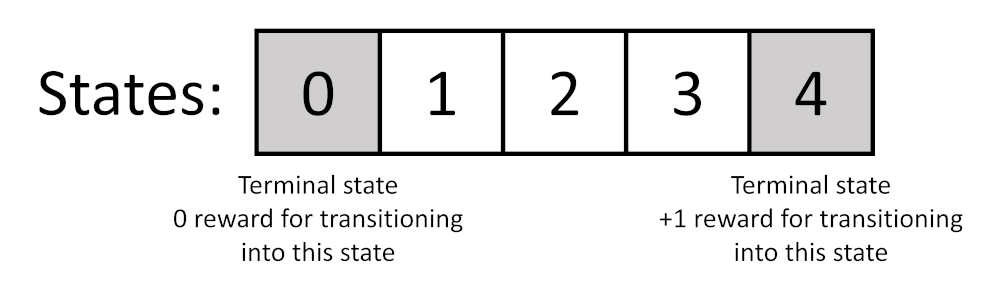
The action space consists of moving left or right. In previous versions of this gridworld, we had a “random slip” element that would make the agent move in the opposite direction 20% of the time. To keep this example simple, we’ll say that this slippage never happens. We’ll also choose a discount factor γ=0.9, an epsilon of ε=0.1 to encourage some exploration, and a learning rate of α=0.1.

Rollout 1

Recall that SARSA and Q-learning are sampled algorithms, which means we update our Q values and the policy at every step. They do not wait for a full episode to end to perform these updates.

At t=0, the agent starts in state 2. The Q-table is all zeros, so the agent chooses right randomly. It takes the right action and observes: R₁=0, S₁=3.

At this point (t=1), the agent can make its update. For SARSA, it needs to know what action it will take next, so it uses ε-greedy on state 3 (still all zeros) to choose A₁, say right. Both SARSA and Q-learning give the same result here since Q(3, right) = 0 and Q(3, left) = 0. The optimal Q* value and the policy are the same.

We calculate the TD error and update the Q value for Q(2, right) for both algorithms.

SARSA:

δ_SARSA = R₁ + γQ(S₁, A₁) – Q(S₀, A₀) = R₁ + γQ(3, right) – Q(2, right) =  0 + 0.9(0) − 0 = 0

Q(2, right) ← Q(2, right) + α(δ_SARSA) = 0 + 0.1(0) = 0

Q-learning:

δ_Q = R₁ + γ max_a Q(S₁, a) – Q(S₀, A₀) = R₁ + γQ(3, right) – Q(2, right) = 0 + 0.9(0) − 0 = 0

Q(2, right) ← Q(2, right) + α(δ_Q) = 0 + 0.1(0) = 0

Q(2, right) stays at 0 for both algorithms.

At t=1, the agent is at S₁=3. It already chose the next action (for SARSA), but Q-learning can choose a different action. Let’s say the agent for both algorithms takes the right action again and ends up in the terminal state. So, R₂=1, S₂=4 (terminal). We can perform another Q update (we set Q(S₂, A₂) = Q(4, any) = 0, as state 4 is terminal):

SARSA:

δ_SARSA = R₂ + γQ(S₂, A₂) – Q(S₁, A₁) = R₂ + γQ(4, any) – Q(3, right) = 1 + 0.9(0) − 0 = 1

Q(3, right) ← Q(3, right) + α(δ_SARSA) = 0 + 0.1(1) = 0.1

Q-learning:

δ_Q = R₂ + γ max_a Q(S₂, a) – Q(S₁, A₁) = R₂ + γQ(4, any) – Q(3, right) = 1 + 0.9(0) − 0 = 1

Q(3, right) ← Q(3, right) + α(δ_Q) = 0 + 0.1(1) = 0.1

At the end of this episode, our Q-table for SARSA and Q-learning are identical because the ε-greedy policy (in SARSA) did not trigger an exploration option different from choosing the action that maximized the Q value (in Q-learning). Here is what the Q-table looks like for both algorithms:

State-Action	SARSA	Q-learning
Q(1, left)	0	0
Q(1, right)	0	0
Q(2, left)	0	0
Q(2, right)	0	0
Q(3, left)	0	0
Q(3, right)	0.1	0.1

0.Note that Q(2, right) was never updated on this rollout because Q(3, right) and Q(3, left) were still at zero (from initialization). The agent didn’t know that going right from state 3 would lead to a reward. It found that out one step later, and that information had not yet propagated back to Q(2, right) by the time the episode ended.

Rollout 2

Using our existing Q-table, let’s perform another rollout.

At t=0, the agent starts from state 2 again (S₀=2). The estimates Q(2, right) and Q(2, left) are both still 0 at this point, so either action is equally likely under the greedy rule. We’ll say that the agent chooses to go right.

The agent takes the action and observes R₁= 0, S₁=3.

Both algorithms can now make their Q update. Let’s say the ε rule fires, and we’ll see how the values can differ. SARSA needs to know what action the agent will actually take next to determine Q(S_t+1, A_t+1). Q-learning will simply choose the max Q value for Q(S_t+1, A_t+1), regardless of what the policy will choose.

From the current Q table, we have Q(3, right) = 0.1 and Q(3, left) = 0. Let’s say that the ε rule will fire for both algorithms, and the agent will select left (despite Q(3, right) being higher). SARSA will use this future action for its Q value update, but Q-learning will use the max_a Q value, regardless of what the actual policy chose.

Let’s see those updates:

SARSA:

δ_SARSA = R₁ + γQ(S₁, A₁) – Q(S₀, A₀) = R₁ + γQ(3, left) – Q(2, right) = 0 + 0.9(0) − 0 = 0

Q(2, right) ← Q(2, right) + α(δ_SARSA) = 0 + 0.1(0) = 0

Q-learning (max_a Q(S₁, a) is max_a (Q(3, right), Q(3, left)), so we choose Q(3, right) here):

δ_Q = R₁ + γ max_a Q(S₁, A₁) – Q(S₀, A₀) = R₁ + γQ(3, right) – Q(2, right) = 0 + 0.9(0.1) − 0 = 0.09

Q(2, right) ← Q(2, right) + α(δ_Q) = 0 + 0.1(0.09) = 0.009

The agent then moves, taking whichever action was chosen. This happens to be left for both algorithms thanks to the ε rule forcing an exploration step.

At t=2, the agent observes R₂=0, S₂=2 from the previous action. It can perform another update. This time, the ε does not fire, so the agent chooses the best Q value. Right now, the Q table has the following values for state 2:

SARSA:

• Q(2, left) = 0
• Q(2, right) = 0

Q-learning:

• Q(2, left) = 0
• Q(2, right) = 0.009

That means, SARSA will randomly choose left or right (both Q values are 0). Q-learning will choose right (higher Q value). You can see how the algorithms begin to diverge here (the agents could potentially take different actions!). To keep this example moving along, let’s say that SARSA will choose right for its next action.

Let’s perform the updates for the previous Q values:

SARSA:

δ_SARSA = R₂ + γQ(S₂, A₂) – Q(S₁, A₁) = R₂ + γQ(2, right) – Q(3, left) = 0 + 0.9(0) − 0 = 0

Q(3, left) ← Q(3, left) + α(δ_SARSA) = 0 + 0.1(0) = 0

Q-learning:

δ_Q = R₂ + γ max_a Q(S₂, a) – Q(S₁, A₁) = R₂ + γQ(2, right) – Q(3, left) = 0 + 0.9(0.009) − 0 = 0.0081

Q(3, left) ← Q(3, left) + α(δ_Q) = 0 + 0.1(0.0081) = 0.00081

The agents for both algorithms take the right action, and at t=3, we get the observation: R₃=0, S₃=3. We do another update:

SARSA:

δ_SARSA = R₃ + γQ(S₃, A₃) – Q(S₂, A₂) = R₃ + γQ(3, right) – Q(2, right) = 0 + 0.9(0.1) − 0 = 0.09

Q(2, right) ← Q(2, right) + α(δ_SARSA) = 0 + 0.1(0.09) = 0.009

Q-learning:

δ_Q = R₃ + γ max_a Q(S₃, a) – Q(S₂, A₂) = R₃ + γQ(3, right) – Q(2, right) = 0 + 0.9(0.1) − 0.009 = 0.081

Q(2, right) ← Q(2, right) + α(δ_Q) = 0.009 + 0.1(0.081) = 0.0171

We repeat this one more time, moving to the right again. At t=4, we end the episode with the episode R₄=1, S₄=4. We can do one more update:

SARSA:

δ_SARSA = R₄ + γQ(S₄, A₄) – Q(S₃, A₃) = R₄ + γQ(4, any) – Q(3, right) = 1 + 0.9(0) − 0.1 = 0.9

Q(3, right) ← Q(3, right) + α(δ_SARSA) = 0.1 + 0.1(0.9) = 0.19

Q-learning:

δ_Q = R₄ + γ max_a Q(S₄, a) – Q(S₃, A₃) = R₄ + γQ(4, any) – Q(3, right) = 1 + 0.9(0.1) − 0.1 = 0.9

Q(3, right) ← Q(3, right) + α(δ_Q) = 0.1 + 0.1(0.9) = 0.19

Here is the updated Q-table after rollout 2:

State-Action	SARSA	Q-learning
Q(1, left)	0	0
Q(1, right)	0	0
Q(2, left)	0	0
Q(2, right)	0.009	0.0171
Q(3, left)	0	0.00081
Q(3, right)	0.19	0.19

We can see how, while similar in many ways, SARSA and Q-learning start to diverge when the evaluation policy chooses an action different from the optimal policy. The clearest sign of divergence is Q(3,left): SARSA still shows zero credit for that state-action pair, while Q-learning has already assigned it a small positive value, even though the agent’s actual next move (right, from state 2) never depended on it. With Q-learning, we can easily explore as needed (e.g. using an ε-greedy policy), and update the estimated Q values as if the optimal actions were chosen.

Limitations of Q-Learning

Like DP, MC, SARSA, and TD(λ), Q-learning is tabular. This means that it must store a separate Q value for every state-action pair. This quickly becomes intractable (or impossible) for large or continuous state spaces.

A key breakthrough for solving the discrete state (or state-action pair) limitation of these algorithms comes from function approximation. Rather than storing a separate Q value for every state (state-action pair), we can approximate V(s) or Q(s,a) with a function: input any real number s or s,a, and you get V or Q out. These functions don’t need to know the actual state or action values; they just need to be approximately correct in order to be useful.

Researchers eventually started to use neural networks as deep, non-linear functions to approximate V(s) or Q(s,a) with amazing results, giving rise to the current trend of Deep Q-Networks (DQN) and deep reinforcement learning (deep RL). Will will dive into DQN starting in the next post.

Conclusion

Q-learning is an online, off-policy TD control algorithm that learns Q* by bootstrapping with the maximum next-state action value, rather than the actual next action as chosen by the policy. The seemingly simple change of replacing the bootstrapped Q(S_t+1, A_t+1) from SARSA with max_a Q(S_t+1, A_t+1) allows the estimation to converge to the real Q* value rather than the ε-greedy approximation.

This one change opened the door to function approximation, which launched the modern era of deep RL. In the next post, we will see how neural networks act as function approximators in DQN, which allows us to start working with large and continuous action spaces, including video games.

If you have any questions or suggestions, please feel free to leave a comment!