Reinforcement learning (RL) is a field of study within machine learning (ML) concerned with developing intelligent agents that take actions in dynamic environments in order to maximize their rewards. RL has gained a lot of popularity in the past few years, most notably in robotics, where big-name companies are using it to create robust locomotion controllers, such as Boston Dynamics’ Spot and Disney’s BDX droid. However, it is incredibly useful in other areas, too, such as driving recommender systems (that recommend products, shows, etc. to customers), replacing A/B testing in marketing (to automatically update content that works well with viewers), and beating human players at video games.
RL has a reputation for being intimidating, and that’s being generous. The math can be quite complex and require many hours struggling with equations to truly grasp what’s going on (I’m speaking from first-hand experience). My hope is to make RL a little more approachable.
I am currently working on a video series that covers the practical aspects of developing RL agents that get deployed to embedded systems. In that series, I plan to gloss over many of the finer details of RL (including the math) in the hopes of making RL more accessible to novices (makers, undergraduate engineers, etc.).
I plan to create a series of blog posts that act as a companion to that series for anyone that wants to really dive into the math behind RL. I’ll start with basic concepts (agent, environment, policy, etc.), introduce fundamental equations (Bellman, TD error, etc.), and build up to how the currently popular Proximal Policy Optimization (PPO) algorithm works.
My goal is to make the math behind RL accessible in as little time as possible so you can build RL agents and frameworks with confidence. If you want to really dive into the math to understand the nuances and sections I might gloss over, I highly recommend the University of Alberta’s Reinforcement Learning Specialization and accompanying RL textbook, which can be downloaded for free from the authors’ site. Note that the textbook is written for graduate-level students, and the math reflects that level of knowledge. If you would like a slightly easier introduction to RL (i.e. spend less time beating your head against the proverbial math wall), I also highly recommend the book Grokking Deep Reinforcement Learning.
Prerequisites
The math covered in this series will be at a graduate level. You should have a firm grasp of statistics, Python programming, and deep learning (neural networks, backpropagation, gradient descent, etc.). I recommend the following materials if you need to brush up on any of these:
- Statistics
- Deep learning
- Python programming
How is RL Different From Other Types of ML?
When you first learn about machine learning (book, course, etc.), you’re often told there are two main forms of ML: supervised and unsupervised learning. In supervised learning, ground-truth labels are provided for the training data, and the training algorithm attempts to minimize the error between the model’s predictions and those labels. In unsupervised learning, no such labels are provided, and the training algorithms attempt to find structures or patterns in the provided data.
With a broad definition of an agent we previously discussed, how does it fit into either supervised or unsupervised learning? The answer is that it doesn’t. RL is often considered a separate subfield from either supervised or unsupervised. When it comes to robotics, the real world is difficult to label, but we can pretty easily craft rewards or penalties.
While RL evolved separately from traditional ML fields, the last few years have seen impressive research gains thanks to the combination of deep learning (i.e. neural networks) with RL (often called deep reinforcement learning).
A Brief History of RL
Before we talk about the core loop of RL, let’s take a brief look at the history of this fascinating field. Feel free to skip this section, but I generally like knowing where something came from!
- RL traces its roots to behavioral psychology, including Pavlov’s classical conditioning (involuntary responses to stimuli) and Skinner’s operant conditioning (voluntary actions reinforced through rewards or punishments)
- 1950s-1960s: Early AI pioneers like Claude Shannon, Arthur Samuel, John McCarthy, and Marvin Minsky laid the groundwork for programs that could learn from experience. Samuel’s checkers-playing program (1959) was an early standout example.
- 1957: Richard Bellman introduced dynamic programming and the Bellman equation, which would become one of the core theoretical pillars of RL
- 1970s-1980s: RL formalized as its own field of study, with the Markov decision process (MDP) providing a mathematical structure for agent-environment interaction. Sutton and Barto were particularly influential in connecting psychological ideas of reward to mathematical learning algorithms.
- 1988-1992: Sutton introduced TD(lambda) and Watkins introduced Q-learning (1989), two fundamentally important algorithms in RL. Gerald Tesauro’s TD-Gammon applied TD learning to reach expert-level backgammon play.
- 1990s: A broader AI funding lull (one of the AI “winters”) slowed RL research significantly
- 2013-2015: Deep learning breakthroughs renewed interest in RL. DeepMind’s DQN learned to play Atari games directly from raw pixel data, launching the deep RL era.
- 2016: Google DeepMind’s AlphaGo defeated Lee Se-dol, one of the world’s top professional Go players, in a result many experts thought was still a decade away
- 2017: OpenAI released Proximal Policy Optimization (PPO), which quickly became one of the most widely used RL algorithms in research and industry, and is the destination of this blog series
- 2019: OpenAI Five defeated professional champions at Dota 2 using PPO at massive scale
Overview of Reinforcement Learning
In RL, you have an “agent,” which is the part of the code or algorithm that takes in an observation from its environment and decides which action should be taken next. If you’re coming from the traditional ML world, you might equate this with a “model” (the mathematical set of equations and trainable parameters that take in some kind of input/reading and returns a prediction), but in the RL world, a “model” is something completely different (it’s related to the environment, something we’ll look at later).
The agent’s goal is to get better over time by interacting with its environment and maximize its rewards (given by the environment) over time.
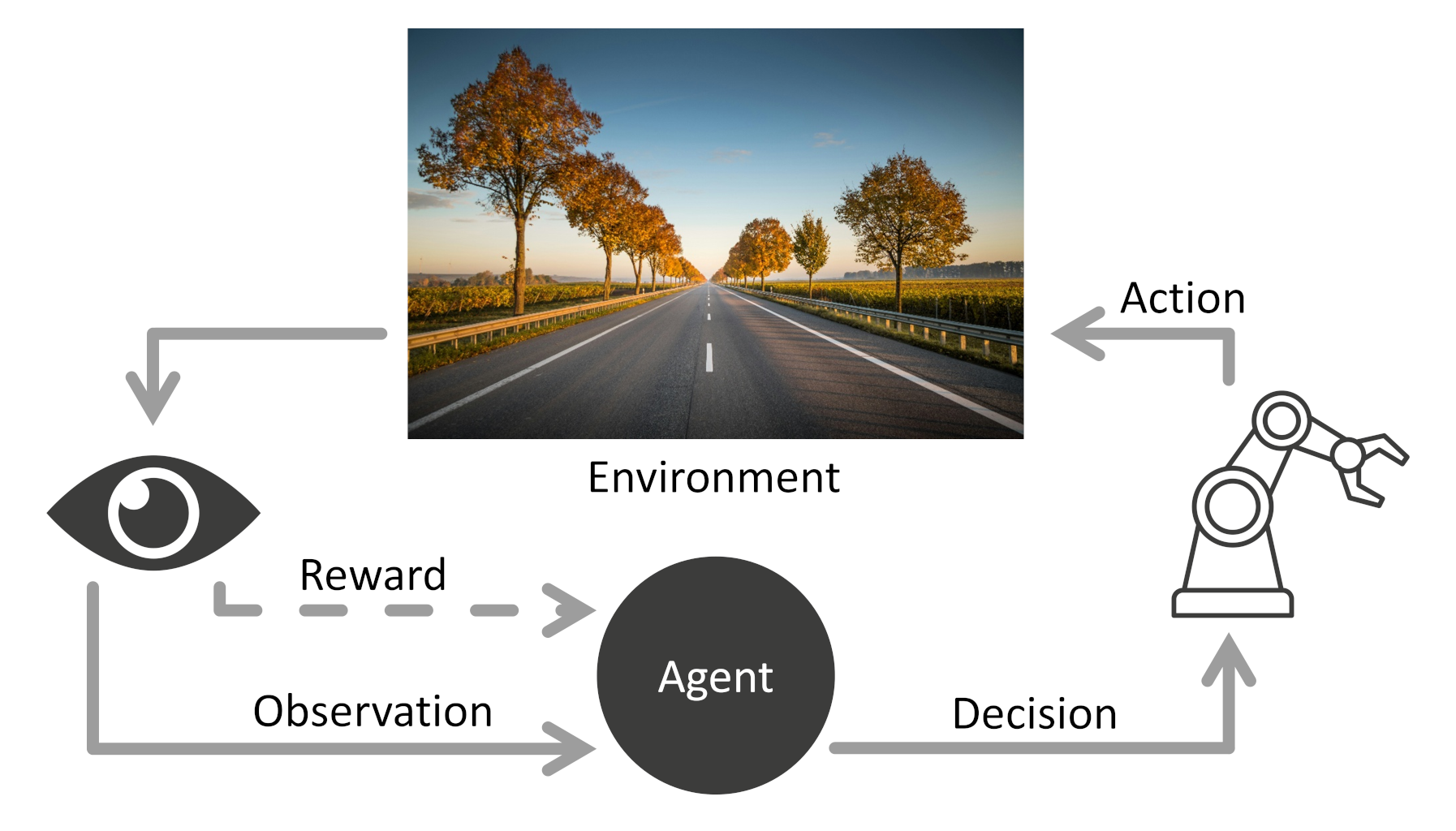
Note that the agent is just the decision maker. Everything else is considered to be part of the “environment.” The environment does include whatever (physical or digital) world the agent inhabits. This could be a chess board, a video game world, or even the real physical world around us. The tricky part is understanding that “everything else” part: any sensors, manipulators, motors, video game controllers, virtual characters, etc. are all considered to be part of the “environment” from the perspective of the agent.
The agent can learn about the environment through one or more observations (e.g. the signals from the sensors, video game pixel data, chess board configuration, etc.). Formally, a set of observations at any given point in time is known as a “state” in the RL world.
Also note that rewards come from the environment. In RL, the agent is incapable of setting its own reward function (at least for now until we get AI agents with the goal-setting capabilities of the prefrontal cortex). As you will see when we develop RL code, the reward function usually lives with the environment portion, and the agent only contains the decision-making functions.
In RL, the agent’s goal is to take the next action that will maximize not just its next reward, but also all future rewards. Because the environments are often dynamic (they change over time or don’t always give the same outcome for each action), it can be difficult to predict what future rewards look like, even if we have a complete model of the environment (e.g. a chess board or video game).
This is where the heavy math and statistics come in: RL algorithms update an agent’s internal parameters to take actions that maximize current and future discounted rewards.
Let’s review the important terms:
- Agent: the part of the algorithm or code that makes decisions
- Environment: everything the agent interacts with
- State: what the agent observes (also known as an “observation”) from the environment
- Action: what the agent can choose to do
- Reward: the feedback signal from the environment
A Concrete Example
Everything we talked about so far was quite theoretical. Let’s take a moment and give a concrete example and apply our new terminology.
Let’s say we want a 2-wheeled robot to balance itself (much like an automated Segway). We’ll start with a bot that has a simple 3-axis accelerometer that gives us how much acceleration the bot feels in the X, Y, and Z dimensions. We use these measurements to calculate the only observation we care about: how much the robot tilts forward or backward (the “pitch”).
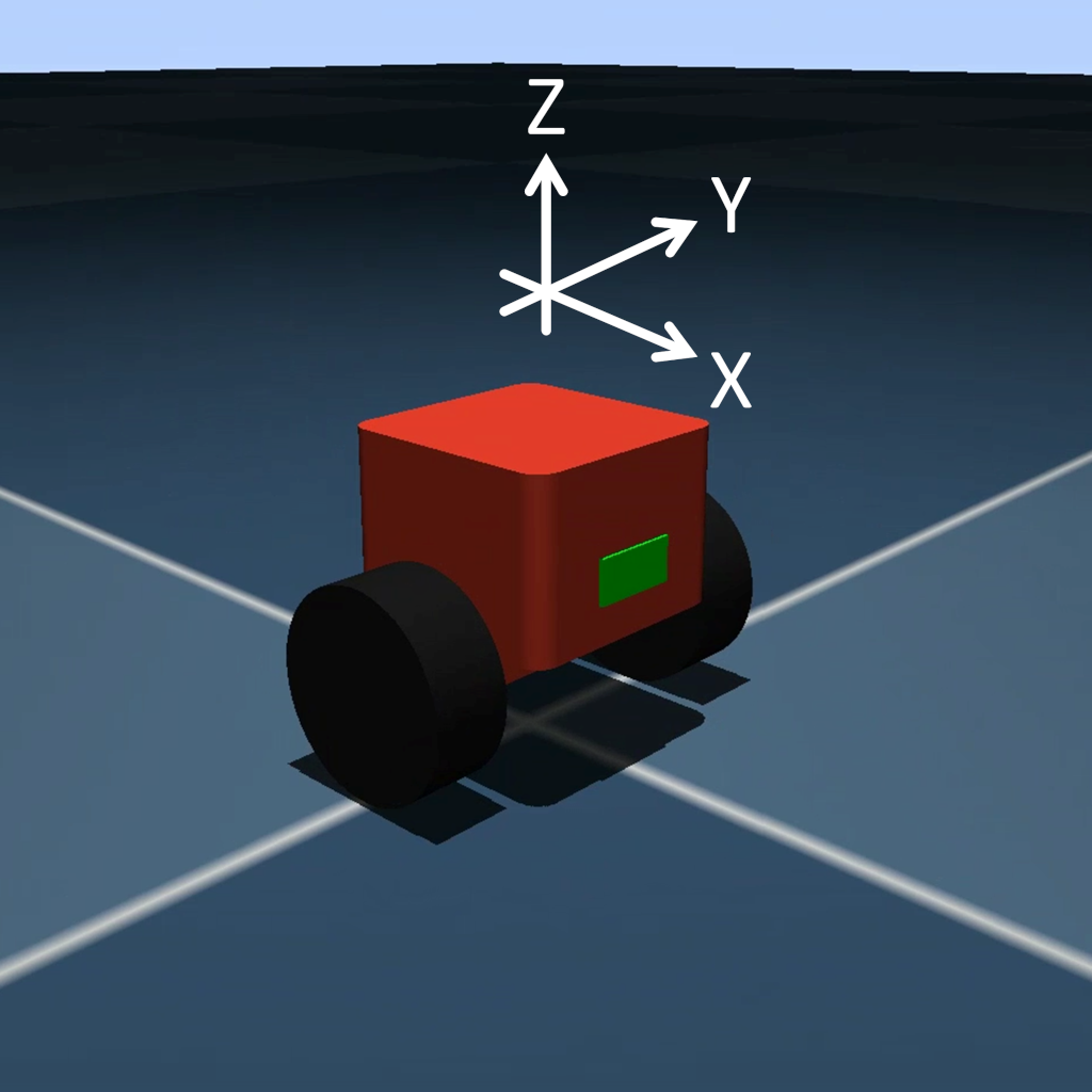
At any given timestep (often referred to as simply a “step”), we can get the state (observation) from the environment.
The agent can only control two things (the “action space”): the power/direction to the left/right motors (given as two normalized floating point values between [-1.0, 1.0]). -1.0 would be full power reverse and 1.0 would be full power forward for a given motor.
We might construct a simple reward function that encourages the bot to stay upright for as long as possible and penalize tipping past a certain point (falling over). A simple reward function might be:
\(r = A – B \cdot \theta^2\)
Where:
- r: the reward for the current timestep
- A: some value for not tipping over (simply staying “alive”), maybe 1.0
- B: coefficient to adjust the importance of the tilt penalty, maybe 5.0
- θ: how much the robot is leaning (radians) away from the vertical (which we assume is 0). We square this, as we only care about the absolute value, and we want to penalize larger pitches more (i.e. the robot is leaning more, and that’s bad).
Note the minus sign. While the agent receives a reward of A at every timestep, it also receives a penalty of B·θ². If the robot is perfectly vertical, it will receive a reward of A (as the penalty would be 0). You can think of this reward like points in a video game: the longer you stay alive, the more points you receive. If you tilt forward or backward while still alive, you lose points.
Let’s say that the interval between timesteps is 0.005 seconds. That means every 5 milliseconds, this reward function is applied. You probably want some kind of total_reward counter that accumulates these rewards at each interval.
If you tip over (say, past 0.5 rad, or about 30 degrees) in either direction, the episode stops and you have to start over. While episodes can continue for infinite time, it’s often easier to reset after some amount of time, even if the robot stayed upright the whole time. So, let’s say the episode resets if you either tip over or if you make it past 30 seconds.
In each episode, you accumulate rewards (based on the reward function). The goal of a good reinforcement learning algorithm is to update the agent in such a way that total_reward is maximized every episode. As you can guess, that can get pretty tricky. In addition to finding, tweaking, and using such an algorithm, you also need to make sure that the reward function correctly captures your intent!
As you might guess, the reward function example we gave is just the beginning. While we reward a bot for staying upright, we have not factored in motion. There’s no penalty for moving around, so the algorithm might produce an agent that wildly drives in circles in quick, jerky motions. While this might accomplish the goal of staying upright (as our reward function dictates), it’s probably not what we imagined when we thought about a balancing robot.
We’ll come back to our reward function in later posts, but for now, you might start thinking about what other observation details you should add to make a balance bot stay in place. Do you need to add additional sensors to the robot to accomplish this?
What RL Is Not Good At (Yet)
Reinforcement learning seems like a magic bullet that allows computer programs to interact with the world and accomplish anything. The truth is that we are nowhere near that reality yet. Thanks to deep RL, we’ve made significant progress in creating complex agents, however, RL has a few shortcomings that you should be aware of.
First, RL often needs lots of interactions to learn, which can take hours or days on expensive hardware. A simple balance bot can be trained on a laptop CPU, but complex motions (e.g. bipedal walking) requires a much more complex setup and time.
Second, most RL algorithms are brittle and subject to large randomness in outcomes. For example, slightly changing a hyperparameter can mean the difference between a working agent and one that just seems to flop around randomly
Third, it’s much easier to train robot agents in simulation (faster execution, parallel environments, ability to speed up time, etc.). However, porting a simulation-trained agent to the real world (known as sim-to-real or sim2real) has its own host of issues and is a current area of active research.
Conclusion
While RL has its limitations, it’s still a rapidly evolving field with great promise for embedded systems and robotics. In the next post, we’ll dive into rewards and how discounted cumulative returns work.
If you plan to follow along, please let me know in the comments! I’ve worked through several courses and books on RL, so this series also gives me a chance to review the fundamentals while working on practical robot examples. I’d love to hear what aspects of RL you find most confusing, or what applications you’re most excited to try.
I first learned about RL more than a decade ago using very difficult hardware and software so I’m looking forward to seeing how you approach this project.
Looking forward for video series