In the third part of this reinforcement learning (RL) series, we’re going to give a formal definition for a policy and then conceptualize how actions and states play out in a trajectory. While we discussed rewards and returns in the previous post, we’re going to see how Markov Decision Processes (MDPs) provide the underlying foundation for RL to work.
In the previous post, we defined rewards and returns, and we showed how the discount factor can account for future uncertainties. We will connect those definitions to the concepts covered in this post in part 4, where we look at value functions.
Policy
A policy is the function that maps environment states to actions. In other words, it is the decision-making part of the agent that accepts a state as an input (remember: a “state” can be a collection of observations, such as sensor readings, camera input, locations of game pieces, etc.) and outputs one or more actions that the agent should take.
As a side note, you will sometimes see “agent” and “policy” used interchangeably in RL literature, but there is a subtle difference between the two. The policy is just the part that maps states to which actions should be taken. The agent, on the other hand, is the full system that includes the policy along with any required value functions (V and/or Q), the learning algorithm used to update the policy and/or value functions, any memory required for storing past episodes (known as a replay buffer), and exploration strategies for trying new actions to learn about the environment.
Mathematically, you will see the policy denoted by π. This can be any function that maps states to actions. For a navigation example, it could be a simple “always turn left” or “if you see an arrow, turn left, else go straight.” As we’ll see later on, such policies can be much more complicated, even including using neural networks that accept observations (the “state”) as inputs and give suggested actions as outputs. Note that both of our simple navigation examples are deterministic. Given a particular state, the same action will be chosen every time.
Much of RL deals with probabilities and stochastic systems, which includes environments and agents that have random variables that can change over time. When we use policies in mathematical equations, you will usually see it denoted as π(a|s). This is a full probability distribution over all possible actions given a particular state s (i.e. a particular set of observations).
Let’s return to our balance bot example. Let’s say we have a very simple observation of “pitch = 0.1 rad” (ignoring the other sensor readings for now). A deterministic policy might say “always apply full motor power in reverse.” A stochastic policy might give a set of possible actions and the probabilities that the agent should choose one of those in order to maximize potential future rewards.
In other words, a policy might take a given state (s) and provide a list of possible actions along with the probability that the agent should choose those actions. If we have a discrete set of actions (i.e. we have a whole number of actions to choose from), given a particular layout of a chessboard (the state), the policy might say something: 90% move pawn A2 to A3, 8% knight B1 to C3, 2% move pawn G2 to G3. The agent would then choose (often based on these percentages) which action to perform.
Since these are probabilities over all possible actions, they must sum to 1.
\(\sum\limits_{a \in \mathcal{A}} \pi(a|s) = 1\)
Let’s take a moment to define action space. It is the set of all valid actions available to an agent in a given environment. Action spaces can be discrete (a finite number of distinct actions, like the chess moves in our example) or continuous (any real value within a range, like the motor torque commands for our balance bot).
If our action space is continuous (i.e. we can apply any real number between -1 and 1 as normalized torque to the motors on our balance bot), then we can integrate over the probability distribution given by the policy to get 1.
\(\int_{a \in \mathcal{A}} \pi(a|s) \, da = 1\)
Note that we will turn back to discrete action spaces in some examples, as it can often be easier to understand the math. However, note that the math still works out if you make the probability distribution slices infinitely small (i.e. you integrate over the curve instead of summing the discrete probabilities).
As you might infer from our discussion, an action space is the set of all valid actions available to an agent in a given environment.
To see how this fits into the bigger picture, recall that the goal of RL is to find a policy π that maximizes the expected return from any starting state. We will spend the next few posts detailing how this idea works mathematically.
Visualizing States and Actions
Over the past few posts, we’ve talked a lot about states and actions, but let’s take a moment to see how they work together to make up an episode. Recall that a state is a set of observations provided by the environment. An action is what the agent decides to do as determined by the policy.
Let’s take a very simplified version of our balance bot. Assume you have a pole attached to a hinge on a cart that can move back and forth. You have three possible actions: do nothing (hold), give the cart a 50 N push to the left, or give the cart a 50 N push to the right.
Let’s take a moment to define observation space. It is the set of all possible observations the agent can receive from the environment.
Your observation space might be the angle of the pole θ (where the pole is upright at θ=0), which would be a continuous observation space. To make this easier, let’s quantize this into a discrete observation space: upright (-0.1 < θ < 0.1 rad), lean left (-0.5 < θ < -0.1), lean right (0.5 > θ > 0.1), and fallen (θ < -0.5 or θ > 0.5).
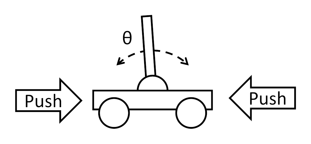
This simplification of the balance bot (or classic inverted pendulum problem) is lovingly known as “cartpole” in the RL world.
We can map the transitions from each state to each other viable state as follows.
Note that all states have arrows pointing at themselves, which means you’re allowed to stay in any given state. The environment cannot jump from “upright” to “fallen” immediately, it must pass through one of the lean left or right states first. Finally, “fallen” is known as a terminal state, which means the episode ends if the pole falls too far. In some diagrams, there would be no arrows coming out of this state. In other cases, you might see such an arrow (often with a reward of 0) going from a terminal state back into itself.
In most cases, when an episode ends due to reaching a terminal state, you would want to restart the episode from the beginning.
In each of the nonterminal states (lean left, upright, lean right), you can perform one of the possible actions (hold, push left, push right). Let’s say that the pole is leaning to the left. We can take one of those actions, but we don’t know which state we’ll end up in next, as this is a stochastic (random) system.
In our simplified system, we’ll say that we don’t have insights into the exact angle of the pole, which would allow us to perfectly model the system behavior thanks to our knowledge of physics. So, the quantization of all angles between -0.1 and -0.5 (as the “lean left”) means that we don’t know exactly where the pole will end up next.
Note that while we’re simplifying the problem here, such models of stochastic systems can also be incredibly useful when we don’t understand the underlying dynamics (e.g. there’s some random wind blowing in cartpole, the rules of some boardgame are unknown, etc.). So, we model these state-action transitions as follows: P(s’ | a, s). This is the probability of ending up in the next state s’ by taking a particular action a when you’re in state s.
Note: we use capital P to denote general probabilities and lowercase p to denote a specific probability. For example, P(s’ | s, a) describes the transition probability function in general, while p(lean left | upright, push right) = 0.3 describes one specific transition probability.
So, let’s say we observe that the pole is leaning to the left. We decide to take the push left action. Our state transition diagram, given this particular combination of state and action, might look like the following diagram.
These demonstrate the randomness of our system. Given our state of “lean left” and our action of “push left,” we have a 60% chance of ending up in “lean right” on the next time step, 20% chance of being “upright,” 10% chance of being in “lean left” again, and 10% chance of terminating the episode in “fallen.” Note that the probabilities must sum to 1 for each state-action pair (i.e. the transition probabilities must sum to 1 for a particular action taken in a particular state).
Here’s what it might look like if we had decided to take the “push right” action instead (from the same “lean left” state).
Notice that we have a much higher chance of ending up in the fallen state now. Intuitively, you can surmise that taking the “push right” action in the “lean left” state is probably the wrong choice.
Markov Decision Process
The current state of RL requires an important, fundamental assumption: the probability of transitioning from one state to the next depends only on the current state and action. This assumes that the state, as given by the observations, does not depend on any other information given by any earlier history of previous states, actions, or transitions.
In other words, states are independent of their history. This is known as the “Markov property,” and is required to model an environment as a Markov Decision Process (MDP). The math we build up to accomplish reinforcement learning requires that the states all have the Markov property. Without it, the math breaks down.
Now, you might be asking: “is it possible to capture history in the states?” and the answer is “yes.” This requires carefully thinking about your observations and state spaces when designing an RL system. For the game of chess, an observation might be a number mapping to a particular configuration of the pieces on the board (which would result in billions of valid states). Another way to do this would be to capture history by encoding the board state across multiple previous timesteps, which is similar to how AlphaZero approaches the problem.
For our cartpole problem, you could use something like pole angular velocity. With an observation space of “pole angle” and “pole angular velocity,” you would have a much easier time figuring out which action to take next, as it would capture some information about the history of where the pole was in the previous few states.
Note that adding this extra piece of observation information increases the complexity of our cartpole system. We would now have even more states: one state for each pair of pole angle and pole angular velocity. Let’s say we’re using our original four pole position observations, and we add three velocity observations: moving to the left, staying still, moving to the right. That gives us 12 total states: lean left and moving left, lean left and staying still, lean left and moving right, upright and moving left, etc.
In our original cartpole example, the observation space consisted of four discrete pole angle bins. By adding angular velocity readings, it expands to twelve discrete states.
While we can capture historical information, the Markov property is not violated in this example. A key takeaway is that you (the designer) should identify observations that give maximum information about the environment while reducing the total number of possible states. More states means more transitions, and more transitions means increased computational complexity when doing the RL math required to find an optimal policy.
With the concept of MDP in place, we can begin to mathematically describe how an agent moves through the environment over time.
Trajectories
A trajectory is one complete path through the MDP in time, from the starting state to a terminal state (assuming there is one). In other words, it’s a sequential list of states, actions, and rewards as the agent moved through the environment. Let’s see how a trajectory is built using our simplified cartpole example.
First, we can map out the state, action, reward possible trajectories in what’s known as a “backup diagram.”
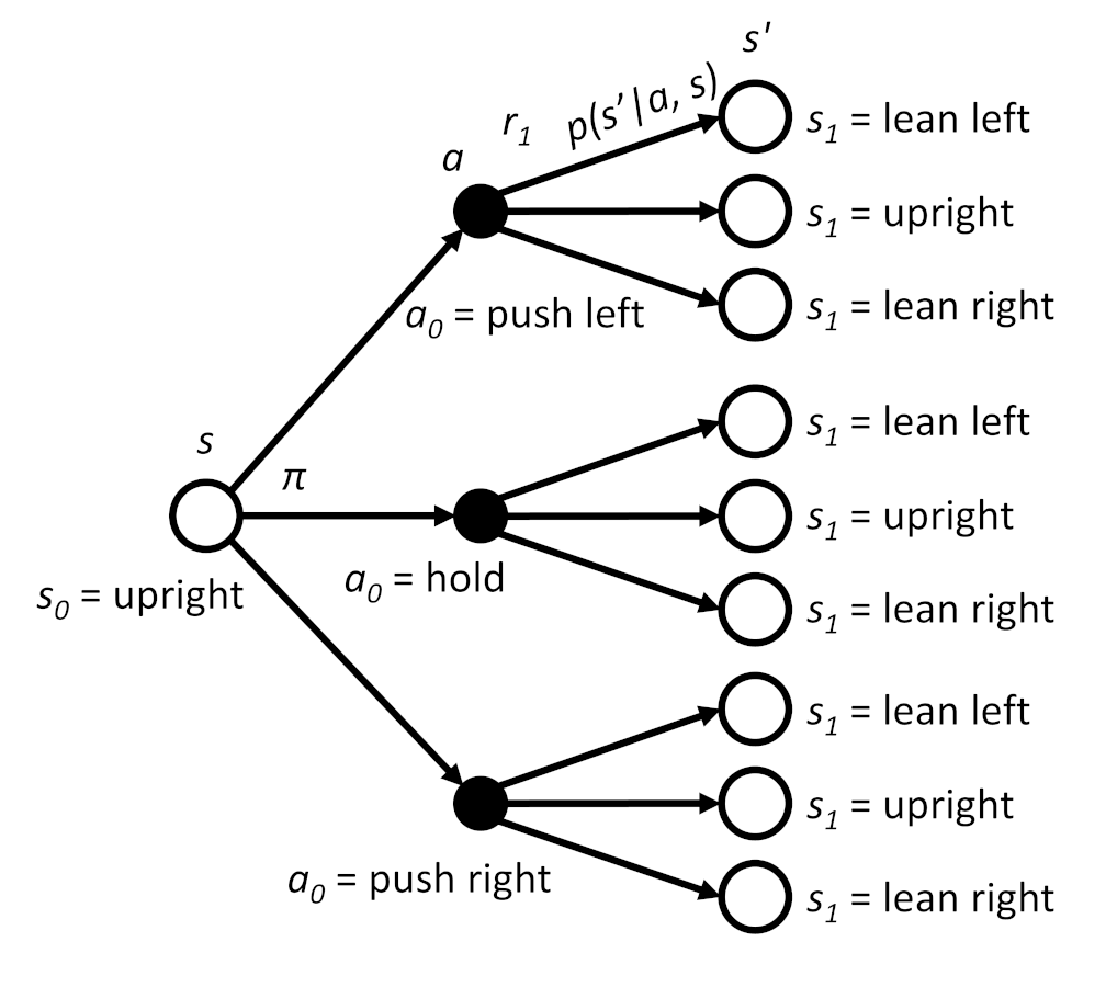
Imagine we start the cartpole somewhere in the upright position: the pole can be randomly leaning anywhere between -0.1 and 0.1 radians. This is considered to be the state at t=0, or s0. We then use policy π to decide which action (a0) to take. Remember: this policy can be anything from “choose an action randomly” to a highly optimized, complex function that chooses an action based on the current set of observations (state).
Whichever action the policy chooses, the environment will give a reward (r) at that timestep. We consider this reward to be part of the next timestep, so the state-action pair of s0 and a0 will result in the reward r1. Then, we transition into the next state (s’). Due to the stochastic nature of the environment, we can end up in any of the four states with a particular probability distribution.
We denote the probability of ending up in state s’ from the state-action pair (a, s) as P(s’ | a, s). Note that we leave out the fallen state as possible s’ states here, as (according to our state diagram earlier), it’s impossible to go immediately from upright to fallen, regardless of the action. In other words, p(fallen | a, upright) = 0. As a result, I left out fallen as a possible state in the diagram.
Let’s say our policy chooses to push the car to the right. We receive the reward r1, and (thanks to the random nature of the transitions) we end up in the lean left state. Once again, our policy looks at the current state and makes a decision about which action to take. This time, it decides to push the cart to the left. We receive a reward (r2) from the environment, and we end up in another state as determined by the transition probability.
We can graph this trajectory (so far) to look something like this:
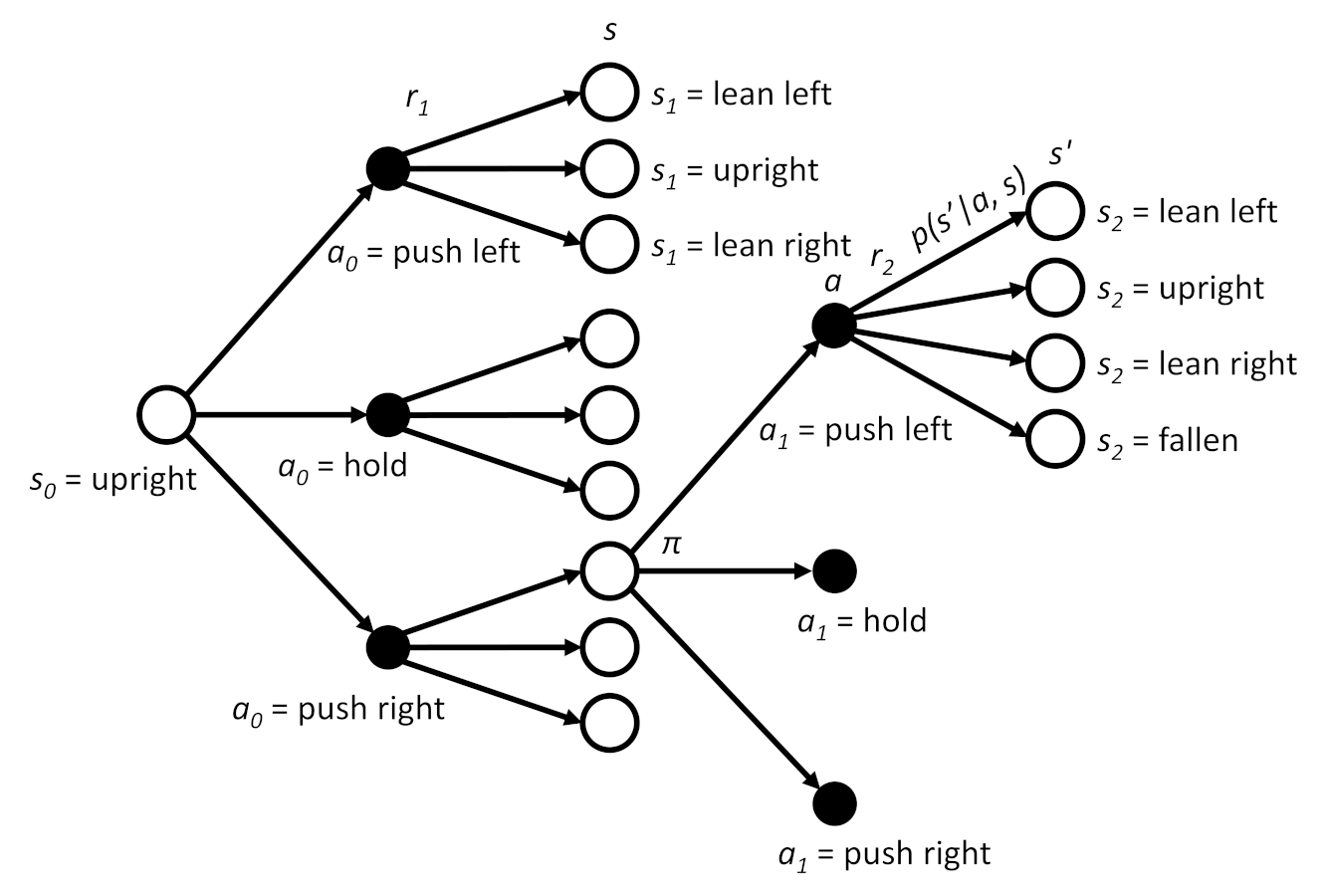
Note that we’re now showing the possibility of ending up in the fallen state here, as that probability is greater than 0 from the lean left state.
This will continue until the pole falls and we reach the terminal state, or until some maximum episode length is reached . We could graph the entire backup diagram for all possible state, action pairs and transitions, and then highlight the actual route the system took during an episode. As you can imagine, the backup diagram for all possible states, actions, and transitions for this cartpole problem would be infinitely large.
However, it is still a useful visualization tool. I like to imagine “standing” at one of the states (the empty circles) and looking out over possible actions, rewards, and transitions going into the future to get a sense of what we’re trying to optimize for the policy. You can also “stand” at different points along the graph. For example, you could stand at one of the filled circles to contemplate the possible reward and transitions after taking that particular action at that particular state (the state-action pair).
If you’re a Dune fan, I imagine this is what Paul Atreides’s prescience ability looks like: being able to foresee the possible states, actions, and outcomes in an ever-widening tree of decisions. The important lesson here is that it takes a mystical foresight ability to fully map out these probabilities. In most RL systems, a complete backup diagram will be impossible to fully realize or the system is simply unknown. As a result, our goal is to learn the system well enough to train a policy that accomplishes our goal. Note that does not mean we always need to fully map out the environment dynamics!
Instead of mapping out the full backup diagram, let’s say we record what actually happens during a particular episode. We could write the trajectory for this episode as follows:
\(\tau = (s_0, a_0, r_1, s_1, a_1, r_2, s_2 \ldots, s_T)\)
In this equation, tau (τ) is the variable used to hold the trajectory. st is the state at time t, at is the action taken from the state at time t, and rt+1 is the reward received from the previous state-action pair at time t. Take note of the timing of the reward: we classify the reward from the starting state (t=0) as r1, the reward from t=1 as r2 and so on.
Remember, this is recorded from a particular episode. Using the example above, s0 = upright, a0 = push right, r1 is whatever reward the environment gave us, s1 = lean left, a1 = push left, r2 is whatever reward the environment gave us, and so on until the pole tips over (ending at sT = fallen).
We can calculate the probability of this particular trajectory occurring (out of all possible trajectories), which is something we’ll need later when calculating expected return. To do this, remember that a policy is the probability of choosing a particular action a at a given state s, which we can write as π(a|s).
We start in a random initial state, the probability of which is given by p(s0). For each step, the probability of ending up in the next state (s’) is given by π(a|s)⋅p(s’|s, a). Recall that we multiply probabilities together to get the joint probability (the probability of two or more events occurring together). In other words, we multiply the probability of our policy taking a particular action given a particular state by the transition probability of moving into the next state s’ given the current state-action pair (s, a).
We continue multiplying these probabilities together to get the probability of a particular trajectory occurring (out of all possible trajectories) given a particular policy π.
\(p(\tau | \pi) = p(s_0) \cdot \pi(a_0 | s_0) \cdot p(s_1 | s_0, a_0) \cdot \pi(a_1 | s_1) \cdot p(s_2 | s_1, a_1) \cdots \pi(a_{T-1} | s_{T-1}) \cdot p(s_T | s_{T-1}, a_{T-1})\)
We can simplify this equation using the product notation:
\(p(\tau | \pi) = p(s_0) \prod\limits_{t=0}^{T-1} \pi(a_t | s_t) \cdot p(s_{t+1} | s_t, a_t)\)
For long trajectories with lots of possible states and actions, you can probably guess that the probability of a given trajectory occurring will be very, very small. The important thing here is that every trajectory will produce a different total episodic return. Even if you’re able to look out into the future and predict these returns to generate a discounted future return, the stochastic nature of this system shows that Gt (discounted future return) must be represented as a random (probabilistic) variable.
Conclusion
We established a few important concepts, including defining a policy (π), a Markov Decision Process, and a trajectory. We assume the Markov property for states in our environment, meaning that a “state” (or “collection of observations”) is independent (i.e. not dependent on the history of previous states). Without this assumption, all of our math going forward breaks down. While non-Markov systems are a fascinating area of research, they’re beyond the scope of this series.
We also looked at how a trajectory is a particular path through all possible states and actions (with rewards given by the environment for a given state, action pair) and formally established the discounted future return Gt as a random variable. We will build on this concept in the next post to derive the value function v(s) and the action-value function q(s, a).
As usual, if you have any questions or comments, please let me know!