Reinforcement Learning Part 11: Deep Q-Networks (DQN)

Previously, we looked at how Q-learning used off-policy temporal difference (TD) updates to converge on an optimal policy. This reinforcement learning (RL) algorithm works surprisingly well, but it requires the environment to have relatively small, discrete state and action spaces. The Q-table can quickly grow to intractable sizes with environments that have a large number of state-action pairs, and the algorithm simply does not work with continuous action spaces.

What if we were to replace the Q lookup table with a parameterized function, such as a neural network (NN)? Rather than recording actual (numerically computed) values of Q(s,a), we could approximate their values. Remember, Q(s,a) is just a function. Ideally, we can give it a state s and an action a, and it should give us a value representing the expected return for that given state-action pair.

In this post, we examine how we can use neural networks to approximate Q(s,a) and find an optimal (local, if not global) policy in a technique called Deep Q-Learning, often referred to as Deep Q-Networks (DQN).

Tables to Function Approximation

In Q-learning, a Q-table stores one entry per (s,a) pair. The algorithm does not consider nor store any relationship between the entries. Q-learning (and other tabular methods) work well in limited circumstances: the state or action space must be discrete, and the number of discrete states/actions must be limited, lest the calculations become intractable.

For example, imagine a simple Atari video game, like Breakout. Atari uses 210×160 pixels, each with 128 colors. You could use the current state of all pixels to create a single entry in a value state (ignoring actions for now). That would give you about 10^71,000 states, which is vastly more state possibilities than atoms in the universe.

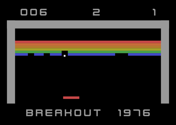
Let’s say you did some preprocessing and hand-crafted a more compact state that denotes the position of the ball, ball direction, paddle position, and brick layout. You could likely end up with a much reduced set of about 10⁴⁰ states. Even with a limited 3 actions per state (move left, move right, hold), you’d need something on the order of 1.2×10⁴¹ bytes, which is many orders of magnitude greater than all the data storage currently available on the Internet. 

This should give you an idea of how Q-learning can quickly become intractable, even with discrete action spaces.

The major breakthrough came in 2013, with DeepMind’s Playing Atari with Deep Reinforcement Learning paper. In it, Mnih et al. successfully demonstrated that Q-tables could be approximated with neural networks. Instead of a lookup table to determine Q(s,a), the expected action values could be approximated using Q(s,a;θ), where θ denotes the set of learnable parameters in a neural network.

This shift from lookup tables to learned function approximation (using deep neural networks) opened the door to a whole new subfield of RL that we now call deep reinforcement learning.

In the paper, the researchers did some preprocessing on the input image to create a scaled and cropped version that stacks 4 frames (to give ball velocity information). The input to the convolutional neural network (CNN) was 84x84x4 as a result. This CNN acted as the function approximation for Q(s,a).

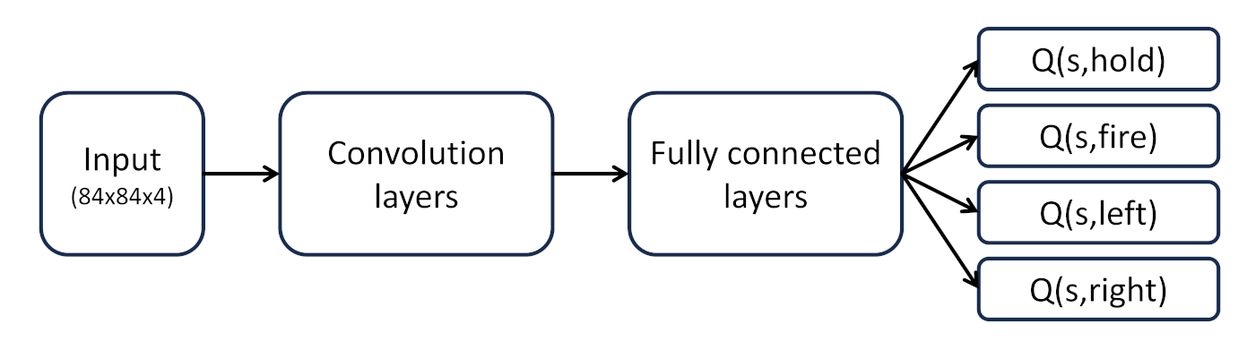
Here’s the trick: the output of the CNN consisted of four nodes, one for each action. So, the CNN would output the estimated Q values for each action given an input state (the four stacked image frames). That means DQN is limited to discrete action spaces, but it can handle large or continuous state (observation) spaces.

Function approximation unlocks continuous state/observation spaces in RL. Previously, we had to use a table to keep track of state or action value estimates, which limited every algorithm we’ve covered so far to discrete spaces. Using a function approximator (a neural network, in this case) means we can input continuous values for our observations directly, since the network generalizes across nearby inputs rather than needing an exact match to something it’s seen before. Keep in mind that this is different from the action space, which still must be discrete for now, as the max operator still needs a finite set of actions to enumerate over, and the NN’s output layer gives us one estimated value per action.

Working With Neural Networks as Function Approximators

In Q-learning, we would update an individual entry in the Q-table after visiting a particular state-action pair, using the experienced, actual reward to perform a TD update. With DQN, instead of overwriting an entry in a table, we adjust the parameters in the neural network using gradient descent. This has the effect of moving the Q(s,a;θ) toward the TD target.

While we showed how CNNs can be used to accept image data as input, the reality is that any nonlinear functions can be used to approximate Q(s,a) (or V(s) if needed). Neural networks are the most popular function approximators right now. The input observation vector does not need to be an image; it could be anything (as we saw in post 1). 

In my RL for robotics project, I used a simple, dense neural network with two hidden layers, each with 48 nodes to act as a function approximator (note: I’m using PPO in this example, which is a bit more complicated, but the idea still stands). In the end, the actor is a single, 3-layer dense network that was easily deployed to an ESP32 microcontroller. 

While researchers are currently looking into using more complex neural network architectures (recurrent neural networks, transformers, etc.), you can do a lot with simple architectures and the right learning algorithm.

Unfortunately, simply substituting neural networks into the Q-learning algorithm as function approximators does not work as expected. We need to make some adjustments to the algorithm to account for the differences between lookup tables and function approximators.

Experience Replay

One of the biggest issues with updating the function approximator every step is that consecutive samples from a single trajectory are highly correlated. Neural networks require independent and identically distributed (i.i.d.) data to ensure that gradient descent converges reliably to a global (or good enough local) optimum. 

To fix this, Long-Ji Lin introduced a technique called experience replay in his 1993 paper Reinforcement Learning for Robots Using Neural Networks. Full transitions (S, A, R, S’) are stored in a replay buffer as the agent performs actions in the environment using an arbitrary policy (random, the policy being updated, ε-greedy, etc.). We can then randomly shuffle this buffer to create uncorrelated (S, A, R, S’) samples that can be used for training the neural network with supervised learning methods.

Q-learning is off-policy, as we saw in part 10, which means we can use max_a Q for the TD target, rather than the action actually taken. This allows us to learn from old experience taken under a stale policy.

In addition to buffering the actual experience, we also need to consider the problem of differentiating with respect to the predictor and target.

Moving Target

To train the neural network, we need to differentiate the loss function with respect to the network’s parameters θ. With DQN, our loss function is just the square of the TD error:

loss = (r + γ · maxa Q(s', a; θ) - Q(s, a; θ))2

We can break apart the TD error into the TD target and the network’s prediction:

target = r + γ · maxa Q(s', a; θ)
prediction = Q(s, a; θ)
loss = (target − prediction)²

Here’s the problem: if we differentiate the loss with respect to θ everywhere it appears (both in the target and the prediction) when performing backpropagation, we end up finding a gradient that nudges those parameters closer together to produce a lower loss next time. As a result, we would move both the target and predictor closer together when performing the gradient descent step to update those same parameters (θ). This, in effect, is like chasing your tail. If we allow the target to move in addition to the predictor, we no longer have a fixed target that we aim for when adjusting the parameters in the predictor. 

Differentiating with respect to all θ is like allowing a student to take a test while editing the answer key. It will often result in Q-values collapsing to the same constants everywhere, meaning the predictor learned nothing useful.

To account for this, we first calculate the target (r + γ · max_a Q(s’, a; θ)) using the current (pre-update) policy and treat it as a constant value. We then differentiate the loss function ((target − Q(s, a; θ))²) with respect to the θ in the prediction value only. In effect, we are breaking θ into two separate sets: one for the target, and one for the predictor. Known as a semi-gradient method, this allows us to keep the target fixed while only moving the parameters in the predictor.

By keeping the target constant, we can then nudge the NN’s set of θ parameters to better predict the target values next time.

DQN Algorithm

With these issues, experience replay and moving target, taken into account, we can formally introduce the full DQN algorithm. 

Initialize:
    Replay buffer D
    Q-network with random weights θ
    Target network weights θ- ← θ
    ε: exploration rate

Loop forever (for each episode):
    Initialize S0
    Loop for each step t:
        Choose At using ε-greedy policy from Q(St, ·; θ)
        Take action At, observe Rt+1, St+1
        Store transition (St, At, Rt+1, St+1) in D
        Sample random minibatch of transitions from D
        For each sampled transition (s, a, r, s'):
            y = r                         if s' is terminal
            y = r + γ maxa Q(s', a; θ-)   otherwise
        Update θ by gradient descent on the mean of (y − Q(s,a;θ))² over the minibatch
        Every N steps: θ- ← θ
        St ← St+1

In this original version, we store every transition and reward (S, A, R, S’) in a replay buffer (D) after taking an action (and observing the environment’s state). Then, after that transition, we would take random transition samples from D to create a minibatch (of e.g. 128 transition samples). These then become our training data for the NN.

For each sampled transition, we would then calculate the constant TD target: r if s’ is terminal and the bootstrapped (r + γ · max_a Q(s’, a; θ^–)) if s’ is not terminal. Note the θ^– notation here. The superscript ‘-’ is used to show that we have to maintain two separate sets of parameters: θ^– is the current (pre-update) parameters used to calculate the (constant) TD target, y. θ, on the other hand, is used to calculate the predicted Q(s,a;θ) value, and the θ should be used as the variable of differentiation when calculating the gradient of the loss function, the mean squared error (MSE) of the TD target minus the predicted Q-value. Note that we take the mean (average) over the full minibatch:

\(L(\boldsymbol{\theta}) = \frac{1}{|B|} \sum_{j \in B} \left( y_j – Q(s_j, a_j; \boldsymbol{\theta}) \right)^2\) 

In most modern implementations of DQN, such as the CleanRL version, you’ll find a few differences and add-ons:

• Limit the size of the replay buffer D. In CleanRL, the buffer defaults to 10,000 samples. Once full, new samples overwrite the oldest samples.
• Let the buffer fill up with data before performing the first NN update.
• Rather than updating the NN every step, let the agent perform some number of actions first, collecting a few (e.g. 10) samples before updating the NN.
• Use Polyak averaging to perform a soft update to the parameters: θ⁻ ← τ · θ + (1 − τ) · θ⁻. The programmer can adjust τ to affect the blending (τ=1.0: hardcopy the full update, τ=0.0 no update, use the old network parameters). It performs slow averaging over time to prevent the network parameters from jumping too quickly in a single update. Side note: if you’ve done any work with sensor fusion or digital signal processing, this is essentially a first-order IIR low-pass filter. 

Limitations of DQN

While DQN proved to be a major breakthrough in the realm of RL, it suffered from a number of limitations. The first is that it worked with discrete action spaces only. As you probably noticed from the neural network diagram, the NN must output a value for each Q value, which means the number of outputs must be equal to the number of actions. This works great for things with simple controls, like video games, but it prevents you from using continuous actions, such as setting the desired speed/torque of a motor.

Additionally, early in training, the Q-values are noisy, due to the NN being initialized with random parameters. As a result, the max_a Q(s,a;θ) operator will often choose values overestimated by the noise, rather than actual best actions (this phenomenon is known as the winner’s curse in statistics). This bias can compound over training since the values get bootstrapped into future targets, resulting in distorted Q-value estimates and inefficient exploration actions.

Like most of the algorithms we’ve studied so far, DQN learns a deterministic policy (e.g. it always chooses the same action given a particular state) thanks to the greedy argmax_a Q(s,a;θ) operation. It is unable to represent a stochastic policy that is capable of randomly choosing an action (e.g. choose “left” 70% of the time and “right” 30% of the time). Stochastic policies allow you to build in exploration (more random in the beginning of training, more deterministic toward the end) and are necessary in some situations, such as a game of Rock-Paper-Scissors where an opponent could learn and exploit a deterministic policy.

Most max-based bootstrapping with ε-greedy policies can be inefficient at discovering good behavior when the reward signals are rare, such as a single reward at the end of a long episode. This method requires lots of random exploration to eventually stumble on the reward, and it can take a while for the reward signal to propagate to earlier actions (as we saw in the Q-learning example).

Sample efficiency is a qualitative measure of how many environment interactions an algorithm needs before it learns a good policy. DQN is generally considered to be sample inefficient, as it often requires thousands or millions of timesteps to converge on a good policy, even for something like a simple Atari game. 

Finally, DQN is notoriously sensitive to small adjustments in its hyperparameters (replay buffer size, learning rate, network architecture, exploration rate, etc.). Getting any one of these wrong can result in an agent that never learns or collapses partway through training (known as catastrophic forgetting). While DQN works great in theory, it requires a lot of fiddling with hyperparameters to get working in practice. 

Researchers have created algorithms over the years to specifically address these problems, like Double DQN. Rather than spend time looking at most of these, we’re going to jump to our next stepping stone in our RL journey, policy gradient methods, as we make our way to PPO. Rather than approximate Q(s,a), these methods directly parameterize and optimize the policy itself. Instead of a network that outputs a value for every action, you get a network that outputs a probability distribution over actions. This shift opens up the possibility of using continuous action spaces and allows for stochastic policies.

Conclusion

We introduced the breakthrough concept of approximating Q-values using neural networks, rather than trying to exactly compute or numerically estimate them using traditional methods. This laid the foundation for later deep RL methods, including the REINFORCE algorithm, which we’ll see in the next post.

If you have any questions or suggestions, please leave a comment!