
In the previous post, we ended with a straightforward application of the policy gradient in the REINFORCE algorithm, which proves to be a useful stepping stone in our deep reinforcement learning (RL) journey. Here, we updated the parameters of the policy approximator (often a neural network) using this formula:
\(\boldsymbol{\theta} \leftarrow \boldsymbol{\theta} + \alpha \cdot \gamma^t \cdot G_t \cdot \nabla_\theta \log \pi(A_t | S_t; \boldsymbol{\theta})\)
Notice that we are using the full return-to-go value of Gt here, which can introduce variance (thus slowing down training by requiring more samples to arrive at better estimated values). The original REINFORCE algorithm also requires full, completed episodes in order to compute Gt via Monte Carlo sampling.
As we’ll see in the rest of the post, we can reduce that variance by using a baseline instead of the raw Gt value. Additionally, by reintroducing bootstrapping, we can open up the possibility of working with continuing (non-terminating) tasks.
This post is a big payoff for the series. We’re going to reference many concepts covered in previous posts, so feel free to go back and review them. Everything we’ve covered so far converges to define the actor-critic architecture, which is the cornerstone for most modern RL algorithms.
The Problem With Raw Returns
We calculate Gt as the return-to-go from timestep t. Gt is a single Monte Carlo (MC) sample, and its magnitude depends on which state the agent happened to be in addition to the action taken. In other words, an action from a promising state produces a large Gt, even when that action was mediocre.
Think about the v(s) table we filled out back in part 6 when we discussed dynamic programming (recall that DP required knowing the state transitions, which allowed us to numerically calculate the state values rather than estimate via MC sampling). Recall that the leftmost and rightmost states were terminal states, with the transition into the leftmost (state 0) offering 0 reward and the transition into the rightmost (state 4) offering a reward of 1.
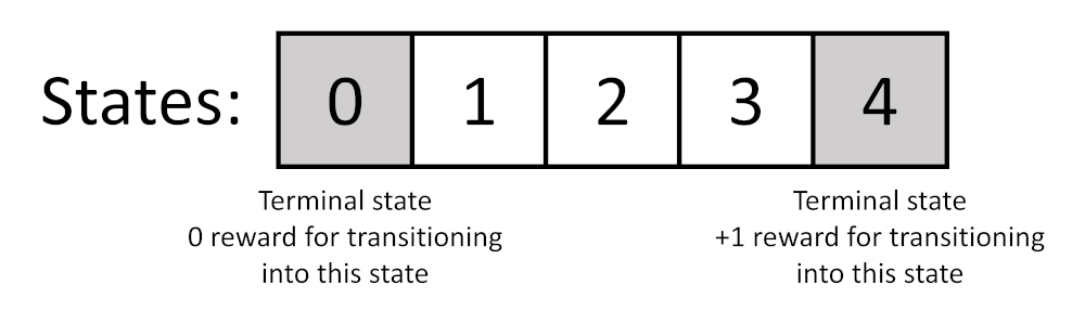
After calculating the values for each state in our 1D gridworld example, we still had decent expected returns. For example, after 3 iterations of DP state 1 had a value of 0.415 and state 2 had a value of 0.576. If an agent was in either of these states, it still looks like there’s a good chance of future rewards. In this particular environment, every reward is either 0 or +1, which means Gt is never negative. Even in environments with negative rewards, we run into the same problem: the magnitude of Gt is mostly determined by which state we’re in, rather than the quality of the actions chosen.
If we were to use a policy gradient method to discover an optimal policy, we’d find that the magnitude of Gt would be the only thing driving the updates in the policy’s parameters, as there are no negative values to drive the policy away from certain actions. We’d eventually settle on a good policy, but it would take a while because only the difference in the Gt values acts as a signal to drive the policy toward one action over another.
In other words, using Gt alone makes the update process increase the probability of mediocre actions simply because things were going well at the time (i.e. the state value looked good regardless of what actions were taken). In post 12, we saw that the gradient term supplies the direction of the parameter update while Gt supplies the magnitude and sign:
\(G_t \cdot \nabla_\theta \log \pi(A_t | S_t; \boldsymbol{\theta})\)
If Gt is always positive, then every action the agent takes gets its probability nudged upward, weighted only by how good the return was. Recall that the policy’s action probabilities (from a given state) must always sum to 1, so they cannot all increase. As a result, the updates end up competing with each other, and the only thing that separates them is that the good action’s Gt was slightly larger. This is a weak signal, which makes training more difficult and often takes longer, requiring more samples.
The Baseline
What if there was a better signal where the sign actually means something? For example, rather than raising the probability of every action (which is what happens in a positive-only return like our gridworld example), we raise the probability of actions that did better than usual from a given state and lower the probability of those that did worse. To do that, we need to compare Gt against some kind of reference point. We’ll call this reference point a baseline.
We’ll use b(s) to refer to some arbitrary baseline from state s. We can then rewrite our update function as follows:
\(\boldsymbol{\theta} \leftarrow \boldsymbol{\theta} + \alpha \cdot \gamma^t \cdot \left( G_t – b(S_t) \right) \cdot \nabla_\theta \log \pi(A_t | S_t; \boldsymbol{\theta})\)
Now, the weight on each update is a difference rather than a raw return. If the episode went better than the baseline suggests it should have, the difference is positive and the action’s probability goes up. If it went worse, the difference is negative and the probability goes down.
For the baseline to work, it can depend on state s, but it cannot depend on any action a. This constraint allows us to subtract the baseline without changing what our gradient ascent is actually optimizing. We want to reduce the variance of the update without affecting the mean; if we changed the mean, we’d be changing the objective of our gradient ascent updates, which we don’t want to do.
Recall from post 12 that this update uses a single sampled episode to estimate a quantity we cannot compute directly. The true gradient is an expectation over all possible trajectories, so if a baseline introduces a bias, it would contribute to the overall average. If we could compute the expectation exactly (rather than estimate via sampling), the update would look like this:
\(\boldsymbol{\theta} \leftarrow \boldsymbol{\theta} + \alpha \cdot \mathbb{E}_{\tau \sim \pi_\theta}\left[ \sum_t \gamma^t \cdot \left( G_t – b(S_t) \right) \cdot \nabla_\theta \log \pi(A_t|S_t;\boldsymbol{\theta}) \right]\)
We can separate the Gt and b(s) terms, thanks to the linearity of expectation.
\(\begin{align*} \mathbb{E}_{\tau \sim \pi_{\theta}}\left[ \sum\limits_{t} \gamma^t \cdot \left( G_t – b(S_t) \right) \cdot \nabla_{\theta} \log \pi(A_t|S_t;\boldsymbol{\theta}) \right] &= \mathbb{E}_{\tau \sim \pi_{\theta}}\left[ \sum\limits_{t} \gamma^t \cdot G_t \cdot \nabla_{\theta} \log \pi(A_t|S_t;\boldsymbol{\theta}) \right] \\ &\quad – \mathbb{E}_{\tau \sim \pi_{\theta}}\left[ \sum\limits_{t} \gamma^t \cdot b(S_t) \cdot \nabla_{\theta} \log \pi(A_t|S_t;\boldsymbol{\theta}) \right] \end{align*}\)
Looking at just the right side of the equation, we can go through a similar set of steps from the post 13 causality proof to first pull out the sum and γt terms from the expectation:
\(\begin{align*}
\mathbb{E}_{\tau \sim \pi_\theta}\left[ \sum\limits_{t} \gamma^t \cdot b(S_t) \cdot \nabla_\theta \log \pi(A_t|S_t;\boldsymbol{\theta}) \right] &= \sum\limits_{t} \mathbb{E}_{\tau \sim \pi_\theta}\left[ \gamma^t \cdot b(S_t) \cdot \nabla_\theta \log \pi(A_t|S_t;\boldsymbol{\theta}) \right] \\
&= \sum\limits_{t} \gamma^t \cdot \mathbb{E}_{\tau \sim \pi_\theta}\left[ b(S_t) \cdot \nabla_\theta \log \pi(A_t|S_t;\boldsymbol{\theta}) \right]
\end{align*}\)
We then separate the trajectory into a prefix (everything before some arbitrary t) and everything after. We can apply the tower rule to rewrite the equation as an expected value of expected values. The prefix ends with St, which is already observed, and b only depends on the state, so b(St) is a fixed value inside the inner expectation, which can be factored out. This is why b(s) cannot depend on any given action: At is still random at this point (i.e. to be chosen by the policy).
\(\begin{align*}
\mathbb{E}_{\tau \sim \pi_\theta}\big[ b(S_t) \cdot \nabla_\theta \log \pi(A_t|S_t;\boldsymbol{\theta}) \big] &= \mathbb{E}_{\text{prefix}}\Big[\, \mathbb{E}\big[ b(S_t) \cdot \nabla_\theta \log \pi(A_t|S_t;\boldsymbol{\theta}) \,\big|\, \text{prefix} \big] \,\Big] \\
&= \mathbb{E}_{\text{prefix}}\Big[\, b(S_t) \cdot \mathbb{E}\big[ \nabla_\theta \log \pi(A_t|S_t;\boldsymbol{\theta}) \,\big|\, \text{prefix} \big] \,\Big]
\end{align*}\)
We can use the chain rule (similar to how we applied it in post 12) to convert π · ∇log π to ∇π. Then, as we showed in post 13, summing over all the probabilities of actions is 1, and the gradient of a constant is 0.
\(\begin{align*}
\mathbb{E}\big[ \nabla_\theta \log \pi(A_t|S_t;\boldsymbol{\theta}) \,\big|\, \text{prefix} \big] &= \sum\limits_{a_t} \pi(a_t|s_t;\boldsymbol{\theta}) \cdot \nabla_\theta \log \pi(a_t|s_t;\boldsymbol{\theta}) \\
&= \sum\limits_{a_t} \nabla_\theta \pi(a_t|s_t;\boldsymbol{\theta}) \\
&= \nabla_\theta \left[ \sum\limits_{a_t} \pi(a_t|s_t;\boldsymbol{\theta}) \right] \\
&= \nabla_\theta [1] = 0
\end{align*}\)
We then substitute this 0 back into the tower rule expression from above, we can show that it does not add anything to the mean:
\(\mathbb{E}_{\tau \sim \pi_\theta}\left[ \sum\limits_{t} \gamma^t \cdot b(S_t) \cdot \nabla_\theta \log \pi(A_t|S_t;\boldsymbol{\theta}) \right] = \sum\limits_{t} \gamma^t \cdot \mathbb{E}_{\text{prefix}}\big[ b(S_t) \cdot 0 \big] = 0\)
While we showed that any arbitrary function can work as a baseline (so long as it does not depend on a), we have not provided a specific baseline.
Choosing a Baseline
Most deep RL applications that rely on baselines use the state value function, v(s). That’s right, it is the same state value function we talked about in post 4. v(s) is “how much return should I expect from a state s at time t under a given policy π.” As a reminder:
\(v_{\pi}(s) = \mathbb{E}_{\pi} \left[ G_t \mid S_t = s \right]\)
As a result, we can then subtract this expected value (a baseline) from the actual total return: Gt – v(s). This tells us how much better or worse the outcome of an action was from the typical expected value (i.e. the baseline).
The issue is, as we have shown in previous posts, that v(s) is difficult to obtain directly, often requiring a full model of the environment (i.e. knowledge of the state transition probabilities). However, we can estimate this value using some arbitrary approximator, similar to how we approximated the policy in post 12.
In many cases, a neural network is used as the approximator for this state value function, which we’ll denote as V(s;φ). Note the capital V to denote the estimated value and the φ term: this is another set of parameters that needs to be learned, or trained, alongside the θ parameters for the policy.
This NN estimator is a relatively straightforward regressor: it accepts an observation vector (i.e. the state) as input, and it gives us an estimated value of that state as an output. Here is a simple 3-layer fully connected NN demonstrating how this might work:

As you can imagine, the inputs can change based on the observation vector chosen, and the architecture can vary depending on the complexity of the environment. This provides yet another set of hyperparameters to be tweaked by the designer of the system.
Let’s see how we can use our new approximator for v(s) as a baseline.
The Advantage Function
The advantage function is a measurement that answers the question, “how much better was a specific action than the policy would do on average from this state?” In other words, we want to compare a real action taken (e.g. from a Monte Carlo sample) to the state value function, v(s). Formally, we define the advantage function as follows:
\(A(s, a) = q_\pi(s, a) – v_\pi(s)\)
As we’ve shown over the series, solving for q(s,a) and v(s) directly is difficult (or impossible) without a full environment model. So, we need to turn to estimation and approximation. First, recall (from post 7) that Gt is a sampled estimate of q(s,a). Second, if we cannot calculate v(s) directly, then we can use our approximator, V(s;φ). We can then define the estimated advantage at timestep t as follows:
\(\hat{A}_t = G_t – V(S_t; \boldsymbol{\phi})\)
Our update rule then becomes:
\(\boldsymbol{\theta} \leftarrow \boldsymbol{\theta} + \alpha \cdot \gamma^t \cdot \hat{A}_t \cdot \nabla_\theta \log \pi(A_t | S_t; \boldsymbol{\theta})\)
We now have a model-free way of updating policy parameters based on sampled episodic returns and an estimated state value. Note that we now have two approximator functions to work with: one that chooses an action based on the observation (state) and another that estimates the value given that same observation.
This combination of REINFORCE with a learned baseline is often called, simply, REINFORCE with Baseline (see an example implementation here). The value network is just recentering the return so the update has an idea of what kind of return to expect from a given state. Note that we still need a complete episode before we can compute Gt in order to make an update. This is the same limitation we ran into with Monte Carlo methods from post 7. We can address this by using the temporal-difference error (TD error) that we saw in part 8.
TD Error
If you recall, the TD error is the difference between the bootstrapped target and our current estimate of the state we just left (V(St)).
\(\delta_t = R_{t+1} + \gamma V(S_{t+1}) – V(S_t)\)
δt gives us a measure of how off the prediction was from the original estimate of the previous state value, or, said differently, it gives a measure of how “surprised” the agent was by what just happened (due to the actual reward just received).
The TD error can act as a valid estimate of the advantage. Instead of relying on the full return Gt, it uses the last reward plus the bootstrapped value of the next state (Rt+1 + γ · V(St+1;φ)). In post 8, V(s) was estimated to fill out a table of state values. Here, we’re using the output of our neural network approximator.
\(\hat{A}_t = \delta_t = R_{t+1} + \gamma \cdot V(S_{t+1}; \boldsymbol{\phi}) – V(S_t; \boldsymbol{\phi})\)
Recall from post 4 that the action value q(s,a) is the expected return after taking action a from state s. We can write that expected return one step at a time: the immediate (actual) reward we received plus the discounted value of whichever state we end up in next.
\(q_\pi(s, a) = \mathbb{E}\big[ R_{t+1} + \gamma \cdot v_\pi(S_{t+1}) \,\big|\, S_t = s, A_t = a \big]\)
This should look familiar: it’s the Bellman equation for q that we saw later in that same post. A single sampled Rt+1 + γ · V(St+1;φ) is just an estimate of q(s,a). As a result, if we subtract v(s), we end up with an estimate for q(s,a) – v(s), which is the definition of the advantage function we just saw.
If δt is positive, it means the action we just took proved to be better (higher reward) than the value estimate from that state. We can use that information to modify the policy (via the θ update formula) to increase the probability of choosing that action in the future. If δt is negative, it means the reward received was worse than expected, and the probability of choosing that action in the future comes down (via the θ update).
This solves the problem of having to wait until the end of a full episode in order to calculate Gt, and we can start calculating and using the advantage as a learning signal on continuing tasks. The tradeoff is that we introduce bias early in the training process. As we saw in post 8, when we substitute the bootstrapped Rt+1 + γ · V(St+1;φ) for Gt, most of the estimate is coming from V(St+1;φ), which itself is an estimate. This makes δt a biased estimate of the advantage early in training, since most of the signal comes from the critic’s own (initially poor) predictions. The bias shrinks as the approximator gets better at predicting state values.
You may also notice that the state value approximator network is regressing toward a target built from its own parameters, which is the moving target problem we saw with DQN in post 11. It’s a less severe problem here, as the network is learning the value of states under the current policy rather than chasing a maximum over actions. As a result, a frozen copy of the network (like DQN’s θ–) is not usually needed here.
Using the value network this way means it’s no longer just a passive reference point. Instead, it is more directly contributing to the learning signal for the policy network. When used this way, the value function is known as a critic.
The Actor-Critic Architecture
The combination of using a function to approximate the policy, π(a|s;θ), and another to approximate the state value, V(s;φ), is known as the actor-critic architecture. Both neural networks are trained at the same time but for different objectives:
- The actor uses the policy gradient (now weighted by the advantage) to become a better decision maker over time
- The critic uses a semi-gradient approach (similar to what DQN uses in part 11) to regress toward its own bootstrapped TD target.
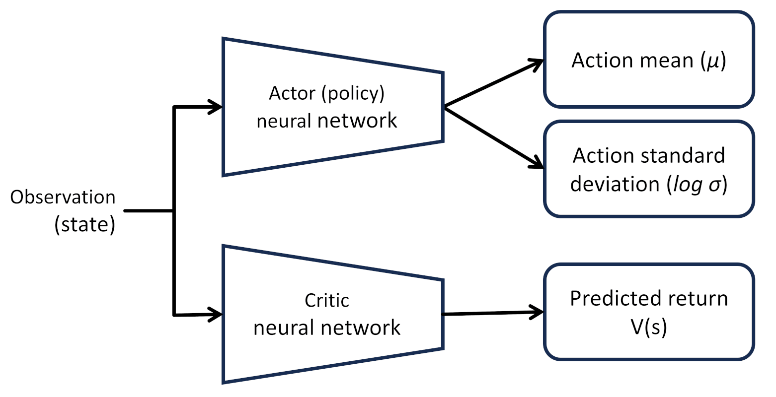
Both networks take the current observation (state) as input. The critic uses it to infer (approximate) the value (total discounted return) of that state. The actor is the policy: it uses the state information to choose an action. More precisely, it generates a mean and standard deviation for a distribution of possible actions, as we showed in part 12. The actor uses the advantage, which is built from the predicted state values from the critic, to update its internal parameters.
One-Step Actor-Critic
We can now devise an algorithm to use this new actor-critic architecture. Note that it requires training two neural networks instead of one: the policy approximator (actor) and the state value approximator (critic).
Initialize:
    Actor (policy) network parameters θ
    Critic (value) network parameters φ
    Step sizes αθ > 0, αφ > 0

Loop forever (each episode):
    Initialize S₀ (first state of the episode)
    I ← 1
    Loop for each step t = 0, 1, 2, … while Sₜ is not terminal:
        Choose Aₜ ~ π(·|Sₜ; θ)
        Take action Aₜ, observe Rₜ₊₁, Sₜ₊₁
        δ ← Rₜ₊₁ + γ · V(Sₜ₊₁; φ) − V(Sₜ; φ) (V(Sₜ₊₁; φ) = 0 if Sₜ₊₁ is terminal)
        φ ← φ + αφ · δ · ∇φ V(Sₜ; φ)
        θ ← θ + αθ · I · δ · ∇θ log π(Aₜ|Sₜ; θ)
        I ← γ · I
In each step, we take an action and observe the reward (R) and the next state (St+1). From this, we compute the single-step advantage, which is the TD error (δ). That error drives the critic’s parameters update (φ), nudging V(s;φ) toward the bootstrapped target. We also use this advantage to update the actor’s parameters (θ). I is simply used to accumulate γ values over time (rather than computing γt at each timestep). We then transition to the next state (St+1) and repeat the process. Rather than wait for an entire episode to complete (as required in REINFORCE), we can now update both actor and critic at every time step!
It might not be obvious from the algorithm, but the critic’s update is doing the same thing DQN’s update did in post 11. There, we defined a TD target, y = R + γ · maxₐ Q(St+1, a; θ⁻), held it constant, and performed gradient descent on the squared difference between it and our prediction. Here, the target is the same bootstrapped quantity we’ve been using for δ:
\(y = R_{t+1} + \gamma \cdot V(S_{t+1}; \boldsymbol{\phi})\)
The loss is the squared TD error, exactly as before, just with V in place of Q:
\(L(\boldsymbol{\phi}) = \left( y – V(S_t; \boldsymbol{\phi}) \right)^2\)
If you differentiate that loss with respect to φ (holding y constant, as we did with the semi-gradient approach in post 11), you get −2 · δₜ · ∇_φ V(Sₜ; φ). Gradient descent means stepping in the opposite direction of the gradient, so the two negatives cancel and the factor of 2 gets absorbed into the learning rate. What’s left is exactly the update in the algorithm above:
\(\boldsymbol{\phi} \leftarrow \boldsymbol{\phi} + \alpha_\phi \cdot \delta_t \cdot \nabla_\phi V(S_t; \boldsymbol{\phi})\)
Most implementations you’ll encounter are written with a loss to minimize rather than a parameter update, since that’s what autograd libraries like PyTorch expect. We’ll see this when we dive into PPO in the next post.
Note that what we’ve shown here is the single-step version of training an actor-critic agent. Much like the TD(0) algorithm from post 8, we only look at the last reward received. In post 9, we introduced TD(λ), which allowed us to use an arbitrary number of rewards after t in order to calculate the TD error. Generalized Advantage Estimation (GAE) uses a similar method of looking at the multi-step advantage function, and it’s something we’ll dig into more in a later post.
Conclusion
We started by identifying two limitations in REINFORCE: the necessity of working with full episode trajectories to calculate Gt and the high variance found in Gt. We introduced a baseline to lower that variance, and choosing v(s) as that baseline gave us the advantage function. However, the advantage function requires computing the state value v(s), which cannot be done directly without knowing the environment dynamics (model). To get around this, we introduced a second neural network to approximate that value, V(s;φ).
We then demonstrated how the bootstrapped TD error worked as an advantage function, which means we could start working in non-terminating environments (i.e. not having to wait for a complete episode to end). When the neural network used to estimate V(s;φ) is used in this manner, it’s often called a critic. Together, the policy approximator and state value approximator (used to estimate the TD error) is called the actor-critic architecture.
Finally, we demonstrated how a one-step actor-critic can be trained. In the next post, we’ll explore how multiple steps can be used to balance bias and variance, along with other techniques, in the proximal policy optimization (PPO) algorithm, which is one of the most popular RL algorithms in use today.
If you have any questions or feedback, please leave a comment below!