
In the previous post, we defined a policy, provided the foundational concept of a Markov Decision Process (MDP), and talked about trajectories. We’re going to combine these concepts with the idea of future discounted returns to create value functions.
We now introduce two new concepts: state-value function (given by V(s)) that attempts to estimate the expected future return from a given state (s), and action-value function (given by Q(s, a)) that attempts to estimate the expected future return from a given state (s) if a particular action (a) is taken.
In order to build these value functions, we need to introduce the concept of expected return, which incorporates probabilities and differs from the previous post’s discussion about discounted future returns.
Expected Return
In the second post, we introduced the discounted return (Gt) that would sum the future rewards (r), each discounted by a factor of γk, where γ is the discount factor (e.g. 0.9) and k is the number of timesteps in the future beyond t.
The issue with this accounting is that we assume we know what the reward will be for future timesteps. In almost every case, we simply cannot know that due to the stochastic and complex nature of the environment: we do not know how the environment might randomly change, react to our actions, or which action an opposing player might choose for a given board game. We also saw that our own policy might be stochastic, meaning we might not even know which actions our own agent will choose.
Due to this uncertainty, we can formalize the definition of discounted return as follows:
\(G_t = R_{t+1} + \gamma R_{t+2} + \gamma^2 R_{t+3} + \cdots = \sum\limits_{k=0}^{\infty} \gamma^k R_{t+k+1}\)
We replace the lowercase r (for a known, given reward) with uppercase R to denote that there is uncertainty involved for that particular reward. As a result, both R and the total Gt are considered random variables (in the world of probability and statistics).
With Gt as a random value, we can estimate its expected value:
\(\mathbb{E}_{\pi}[G_t]\)
As a reminder, to calculate the expected value of a random variable, you multiply each possible value it could take by the probability of that value occurring, then sum everything up . So, to calculate the expected return, we substitute in our definition of Gt:
\(\mathbb{E}{\pi}[G_t] = \mathbb{E}{\pi} \left[ \sum\limits_{k=0}^{\infty} \gamma^k R_{t+k+1} \right]\)
Note that we add the subscript π to denote that this is the expected return for a given policy. If our policy changes, then the expected return also changes.
So, how do we calculate this expected value? Let’s imagine our simplified cartpole example from part 3.
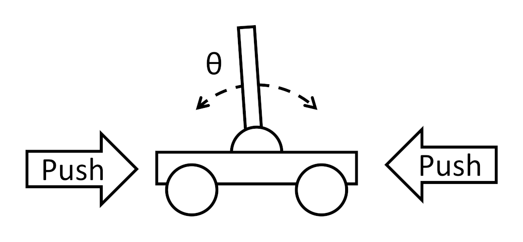
The motor and sensor noise, random starting position (within the “upright” state), state transition randomness, etc. cause the trajectory through the states to be somewhat random, even as we try to apply policy π to keep the pole upright. All of these sources of randomness mean that even starting from the same initial state and following the same policy, each episode will produce a different trajectory τ through the states.
\(\tau = (s_0, a_0, r_1, s_1, a_1, r_2, s_2, \ldots, s_T)\)
In other words, there are many possible trajectories through the states with a given policy. The probability of a particular trajectory is given by p(τ|π), which is often a very, very small number. If we add up all the possible trajectory probabilities, we should get 1.
\(\sum\limits_{\tau} p(\tau | \pi) = 1\)
Now, if we multiply the probability of that one trajectory with the discounted return Gt for that trajectory, we get that trajectory’s contribution to the expected return. Summing all these contributions across all possible trajectories gives us the full expected return.
\(\mathbb{E}_{\pi}[G_t] = \sum\limits_{\tau}p(\tau | \pi) \cdot G_t(\tau)\)
You can substitute the definitions for p(τ|π) and Gt to get a fully expanded version of expected return.
\(\mathbb{E}{\pi}[G_t] = \sum\limits_{\tau} \left[ p(s_0) \prod\limits_{t=0}^{T-1} \pi(a_t | s_t) \cdot p(s_{t+1} | s_t, a_t) \right] \cdot \left[ \sum\limits_{k=0}^{\infty} \gamma^k R_{t+k+1} \right]\)
To get a sense of what this entails, imagine “standing” at the initial state (s0) and imagine one possible trajectory through the states (until the terminal state sT). Figure out the probability of that one trajectory and multiply it by the total discounted return for that trajectory. Now, imagine another possible trajectory through the states, calculate the probability of that second trajectory and multiply it by that trajectory’s discounted return. Repeat this process for all trajectories and continue summing discounted reward for that trajectory weighted by the probability of that trajectory. The final sum is your expected return.
Note that the number of possible trajectories in any sufficiently complex task with discrete actions and states will measure in the millions or billions. Introducing continuous actions or states means that the number of possible trajectories becomes infinite. Manually calculating the expected return quickly becomes intractable. In practice, rather than summing over all possible trajectories, we estimate the expected return using value functions, which give us a tractable shortcut.
State-Value Function
Instead of standing at the initial state s0 to figure out the expected return, what happens if we stood at some arbitrary state in that trajectory? You could calculate the expected return from here if we followed policy π.
Here’s the neat part: due to the Markov property, we must assume that any given state must fully encode all of the required information about that state, regardless of when or how the agent arrived there. The expected future return from state s depends only on the policy π and state s itself, not the history of actions that lead us to state s. In case you were wondering where the MDP assumption mattered, here it is. The math going forward breaks down without the Markov property.
Put another way: it does not matter if you imagine yourself standing at some state s along the trajectory or on the state flow diagram. The possible actions, rewards, and future states are exactly the same. Without the Markov property, the history of getting to the current state s might mean those probabilities change (i.e. the next step in the trajectory and the next step in the flow diagram might be different).
So now, we can write this expected return as given from a particular state s as the following function:
\(v_{\pi}(s) = \mathbb{E}_{\pi} \left[ G_t \mid S_t = s \right]\)
We can substitute our definitions of expected return to expand the equation to the following, which is known as the Bellman equation for vπ (named after Richard E. Bellman).
\(v_{\pi}(s) = \sum\limits_{a} \pi(a|s) \sum\limits_{s’,r} p(s’, r | s, a) \left[ r + \gamma v_{\pi}(s’) \right]\)
Let’s take a moment to talk about what’s going on here. First, instead of starting at the initial state s0, we start at any arbitrary state s. We want to calculate the value we expect to receive from that particular state under a given policy, which we denote as vπ(s). We first sum all of the probabilities of taking an action from that state, which remember, is given by our policy π(a|s). Recall that if we just sum up all the probabilities of taking the different actions from state s, it should equal 1.
To get the expected value, we multiply each probability of taking a particular action with the expected return from that next state. Note that this is recursive: we use the state-value function as given from the next state, vπ(s’) to calculate the state-value function in state s.
That means we need to sum across all probabilities of receiving reward r and transitioning into the next state s’. If there is only one reward for any given action from state s, then this would be a single summation: all possible next states s’ with the rewards for those transitions. However, rewards can also be stochastic. If you have multiple possible rewards for a given action from a given state, then you need to sum across those, too.
Now we have a double summation: we need to calculate the expected value of the reward (r) plus the discounted expected return from the next state vπ(s’), weighted by the joint probability of receiving that reward r and moving into state s’. That produces the expected discounted return after having taken action a. We then weight this by the probability of taking action a and sum all those weighted expected returns together. This provides us with the expected value from state s, which we call the state-value function.
State-Value Example
Let’s look at our cartpole example again. I’ve added example rewards for each of the transitions. Moving into an upright position, the agent is rewarded 1 point. Moving into either lean left or lean right, the agent is rewarded 0.5 points. If the agent falls, it is rewarded no points, and the episode ends.

Note that this is a very simplified reward structure. Rewards can be stochastic, meaning they can be random given a particular action and transition. The state-value function captures this stochastic nature when you sum across all possible rewards and next states (i.e. one action, multiple possible rewards for that action, and from each of those, multiple possible transitions to new states). For now, we assume they are deterministic to keep this example simple.
Next, let’s say we know the transition probabilities for each state-action pair. I’ll diagram all the possible state transitions from the “lean left” state for each possible action (hold, push left, push right).
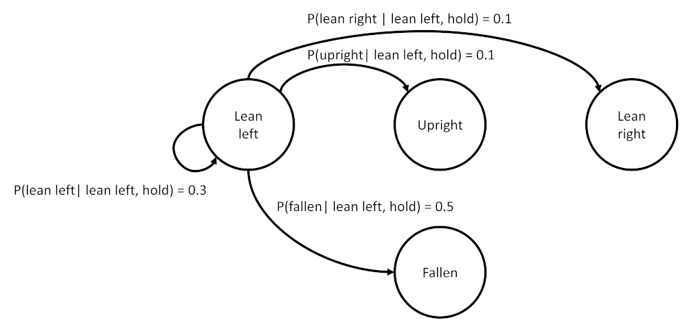
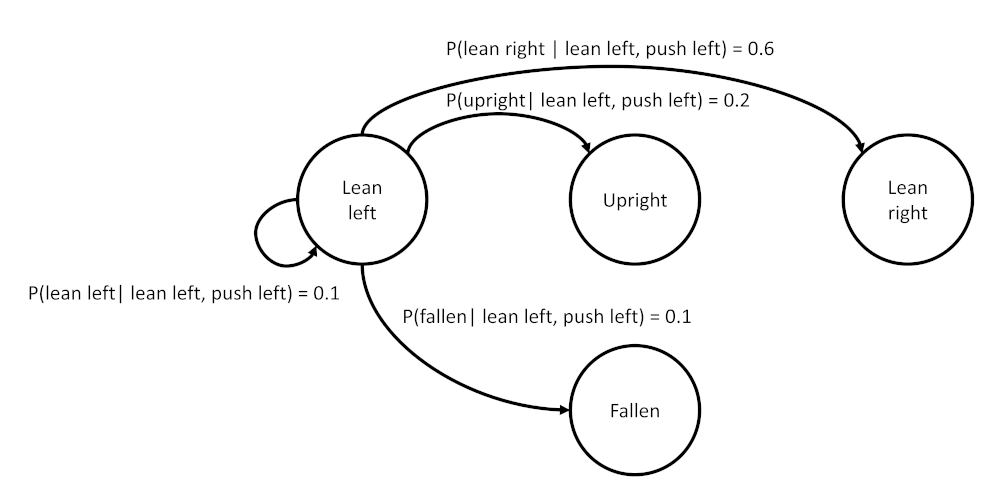
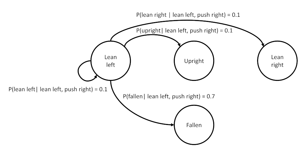
Now, let’s say we know the values at each state, except for the “lean left” state. Remember: the “value” in this sense is the expected discounted return from being in that particular state. Also, these values are for a given policy.
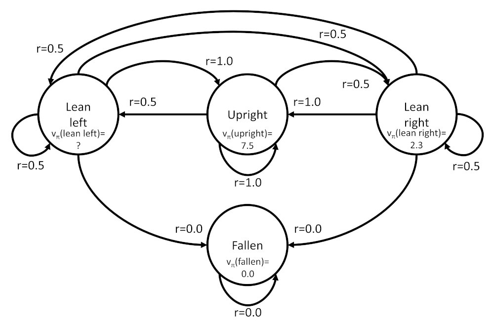
We can use this information to calculate the expected value when the agent is in the “lean left” state. Let’s say that we have a discount factor of γ=0.9 and our simple policy has the following probabilities of choosing a particular action in the “lean left” state:
- π(hold | lean left) = p(hold | lean left) = 0.3
- π(push left | lean left) = p(push left | lean left) = 0.7
- π(push right | lean left) = p(push right | lean right) = 0
Now, we can plug this information into our state-value function to calculate a definite value:
vπ(lean left) = π(hold | lean left) ⋅ (p(s’=lean left | lean left, hold) ⋅ (r + γ ⋅ vπ(lean left)) + p(s’=fallen | lean left, hold) ⋅ (r + γ ⋅ vπ(fallen)) + p(s’=upright | lean left, hold) ⋅ (r + γ ⋅ vπ(upright)) + p(s’=lean right | lean left, hold) ⋅ (r + γ ⋅ vπ(lean right))) + …
vπ(lean left) = 0.3 ⋅ (0.3 ⋅ (0.5 + 0.9 ⋅ vπ(lean left)) + 0.5 ⋅ (0 + 0.9 ⋅ 0) + 0.1 ⋅ (1 + 0.9 ⋅ 7.5) + 0.1 ⋅ (0.5 + 0.9 ⋅ 2.3)) + 0.7 ⋅ (0.1 ⋅ (0.5 + 0.9 ⋅ vπ(lean left)) + 0.1 ⋅ (0 + 0.9 ⋅ 0) + 0.2 ⋅ (1 + 0.9 ⋅ 7.5) + 0.6 ⋅ (0.5 + 0.9 ⋅ 2.3)) + 0 ⋅ (…)
Note that I didn’t write out all the transition and reward probabilities for the “push right” case, as our current policy has a 0% chance of choosing that action.
So, we can factor all of the values to get this simplified version:
vπ(lean left) = 0.045 + 0.081 ⋅ vπ(lean left) + 0 + 0.03 + 0.2025 + 0.015 + 0.0621 + 0.035 + 0.063 ⋅ vπ(lean left) + 0 + 0.14 + 0.945 + 0.21 + 0.8694 + 0
Then we solve for vπ(lean left):
vπ(lean left) ≈ 2.98
While we won’t necessarily know the values of the individual states, I hope this example helps you understand the math a little better for how the state-value function is defined.
Rather than assigning a value to each state, we also have the option to assign a value to an action taken from a particular state (known as a state-action pair). In the next section, we’ll see how that value is calculated (and how it’s different from the state-value function).
Action-Value Function
Instead of “standing” at a state and figuring out the expected return from that state (i.e. the state-value function), imagine that you just took action a from state s (whether you are following policy π or not), and you are about to receive a reward and transition to the next state.
Take a look at the following backup diagram for our simplistic cartpole example. We just performed the action “push right” from the state “upright.” This is the state-action pair: the specific combination of an action taken from a particular state. We’re now where the arrow points, ready to receive a reward and (stochastically) move to a new state.
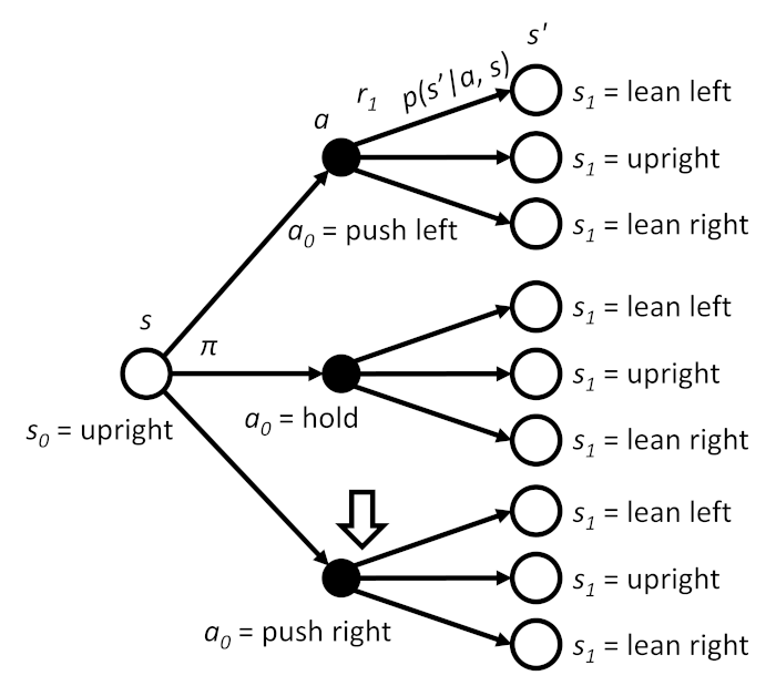
What is the expected return at this point? It’s similar to the state-value function, except that we calculate the discounted return, Gt, given the state-action pair (rather than just the state, like we saw for the state-value function).
\(q_{\pi}(s,a) = \mathbb{E}_{\pi} \left[ G_t \mid S_t = s, A_t = a \right]\)
This is known as the action-value function, and we can use it in a similar fashion to the state-value function. Sometimes, a particular RL algorithm will use one over the other, so it’s important to understand both. For example, Q-learning uses the action-value function directly, while some policy gradient methods rely primarily on the state-value function.
If we substitute in the definition of E[Gt], we get the fully expanded version, known as the Bellman equation for qπ. It’s similar to the Bellman equation for vπ, but we don’t need to sum across the possible policy actions in the beginning (as we’ve already decided on an action from state s). Once again, notice that it is recursive: the current value of qπ(s,a) is dependent on the next action-value given by qπ(s’,a’).
\(q_{\pi}(s,a) = \sum\limits_{s’,r} p(s’, r | s, a) \left[ r + \gamma \sum\limits_{a’} \pi(a’|s’) q_{\pi}(s’, a’) \right]\)
Note that summing over all possible qπ(s,a) values weighted by the probabilities of taking an action in state s (also known as the “policy”) is equal to the state value given by vπ(s). Put mathematically:
\(v_{\pi}(s) = \sum\limits_{a} \pi(a|s) \cdot q_{\pi}(s,a)\)
That means you can rewrite the Bellman equation for qπ as follows, which helps express q in terms of v and vice versa.
\(q_{\pi}(s,a) = \sum\limits_{s’,r} p(s’, r | s, a) \left[ r + \gamma v_{\pi}(s’) \right]\)
Action-Value Example
Given the state values we calculated from the state-value example section, can we figure out the action-value after taking the “push left” action from the “lean left” state?
First, we can fully expand the Bellman equation for qπ using our known probabilities and rewards:
qπ(lean left, push left) = p(s’=lean left | lean left, push left) ⋅ (r + γ ⋅ vπ(lean left)) + p(s’=fallen | lean left, push left) ⋅ (r + γ ⋅ vπ(fallen)) + p(s’=upright | lean left, push left) ⋅ (r + γ ⋅ vπ(upright)) + p(s’=lean right | lean left, push left) ⋅ (r + γ ⋅ vπ(lean right))
We can then plug in the numbers from the previous example:
qπ(lean left, push left) = 0.1 ⋅ (0.5 + 0.9 ⋅ 2.98) + 0.1 ⋅ (0 + 0.9 ⋅ 0) + 0.2 ⋅ (1.0 + 0.9 ⋅ 7.5) + 0.6 ⋅ (0.5 + 0.9 ⋅ 2.3)
qπ(lean left, push left) ≈ 3.41
This gives us the expected return for having taken the “push left” action from the “lean left” state.
We can use this result alongside our earlier vπ(lean left) calculation to verify the relationship between v and q. Using the very simple policy we outlined earlier (at least for taking actions from the “lean left” state), we can use the definition of v (in terms of q) to figure out q(lean left, hold). Note that this only works because we assume π(push right | lean left) = 0, which leaves us with only one variable to determine.
vπ(lean left) = π(hold | lean left) ⋅ qπ(lean left, hold) + π(push left | lean left) ⋅ qπ(lean left, push left) + π(push right | lean left) ⋅ qπ(lean left, push right)
2.98 = 0.3 ⋅ qπ(lean left, hold) + 0.7 ⋅ 3.41 + 0 ⋅ qπ(lean left, push right)
qπ(lean left, hold) ≈ 1.98
This should help make the intuition clearer: we expect to get more value from taking the “push left” action from the “lean left” state (hopefully helping the pole stay upright longer) than if we take the “hold” action.
Conclusion
In this post, we formalized the connection between probability and value estimation: what it means to work with an expected value in terms of our discounted return. We then applied this definition to two important equations, the state-value function and the action-value function, which helps establish how we determine expected future values from particular states and after taking particular actions. By now, you should have a good sense of how v and q are calculated and how they relate to each other.
In the next post, we will introduce the Bellman optimality equations for v and q, which define what the optimal value functions look like and set the stage for the learning algorithms we’ll cover in subsequent posts.