
In the previous post, we introduced the breakthrough concept of combining deep learning and reinforcement learning (RL). Instead of recording estimated Q-values in a table, which is intractable for large or continuous state spaces, we approximated those Q-values using a neural network. This simple act spawned the current generation of deep RL, paving the way for more complex algorithms, such as proximal policy optimization (PPO).
We introduced the deep Q-network (DQN) algorithm, which approximated Q-values using a set of trainable parameters, θ, in a neural network. This network would give us a set of Q-values for each action, a, given a state, s: Q(s,a;θ). In other words, you could input your observation (s) into the neural network and get a set of Q-values, one for each action, as the output. We could then use the greedy method to choose the highest Q-value as our intended action, often with a random chance to perform a different action (ε) to encourage exploration.
DQN suffers from a number of limitations. It works with discrete action spaces only, the ε-greedy policy of maxa Q(s,a;θ) would often choose values overestimated by the noise, and it learned a deterministic policy only (ignoring the random ε chance to explore). DQN is also sample inefficient compared to other, later deep RL algorithms, and it is notoriously sensitive to slight adjustments in hyperparameters. Other algorithms, like Double DQN, throughout the years would address these problems, but in our steady march toward PPO, we’re going to focus on the next milestone: policy gradient
We’re going to spend most of our time deriving the policy gradient theorem, as it’s an important building block for understanding later deep RL algorithms. In the next post, we’ll use the REINFORCE algorithm as a brief example to demonstrate how the policy gradient is used to optimize a policy.
Parameterizing the Policy
Up till now, we’ve been relying on the simple greedy policy: choose the action with the highest Q-value. We slightly modified that policy with the option to randomly choose a different action with ε probability, known as the ε-greedy policy. Both policies require having a discrete set of actions to choose from in order for the maxa Q(s,a) or maxa Q(s,a;θ) operations to work properly. This inherently limited us to discrete action spaces.
To move to very large or continuous action spaces, we need another method of choosing the best action. Just like we approximated Q(s,a), we can approximate the policy as well. We can use some arbitrary function for our policy, which we’ve always defined as π(a|s). What if we used some complex, non-linear function to approximate this function, say a neural network (NN) with a set of parameters θ?
While you could theoretically use any function to approximate π, neural networks have been used for a while in policy approximation, as they offer sufficient complexity and trainable parameters. We will continue to focus on using them in our posts, but know there is continued research into using other functions as policy approximators.
Recall that π(a|s) is the probability of choosing action a given state s, and all the probabilities (for a given state) should sum to 1. That means π is a probability distribution. Our approximation function should take a state (i.e. an observation vector) as an input and output a probability distribution. Here is a simple three-layer NN as an example that does exactly that:

Note: this diagram uses the hyperbolic tangent (tanh) activation function for the hidden layers, matching CleanRL’s PPO default. Bounded activations (e.g. tanh) tend to produce more stable policy training in practice, rather than e.g. ReLU.
This gives us a Gaussian probability distribution for a single action. Most policy approximators use log σ as the standard deviation output head. While you could estimate σ directly, standard deviation must be strictly positive, and it can be difficult to enforce NNs to output positive values all the time.
If you take the cartpole example from post 3, you can imagine that we now have the option of sampling a continuous action from this distribution, rather than relying on the discrete “hold,” “push left,” “push right.” For example, we might sample from this distribution to get the desired action: exactly 0 would be “hold,” -3.7 might be a large “push left,” and 0.2 might be a small “push right.”
In practice, the action space is normalized to a fixed range like [-1, 1] and clipped after sampling. The network isn’t forced to output values in that range, but gradient descent naturally settles it there, since values clipped beyond that range have no effect on reward.
The simple example showed how a single action might work, as we would have for cartpole. You have the option of using a larger action space. For example, the balance bot we talked about in the first post has two action outputs to consider: a normalized [-1, 1] control for the left motor and a normalized [-1, 1] control for the right motor. We can just add more heads to the NN as follows:
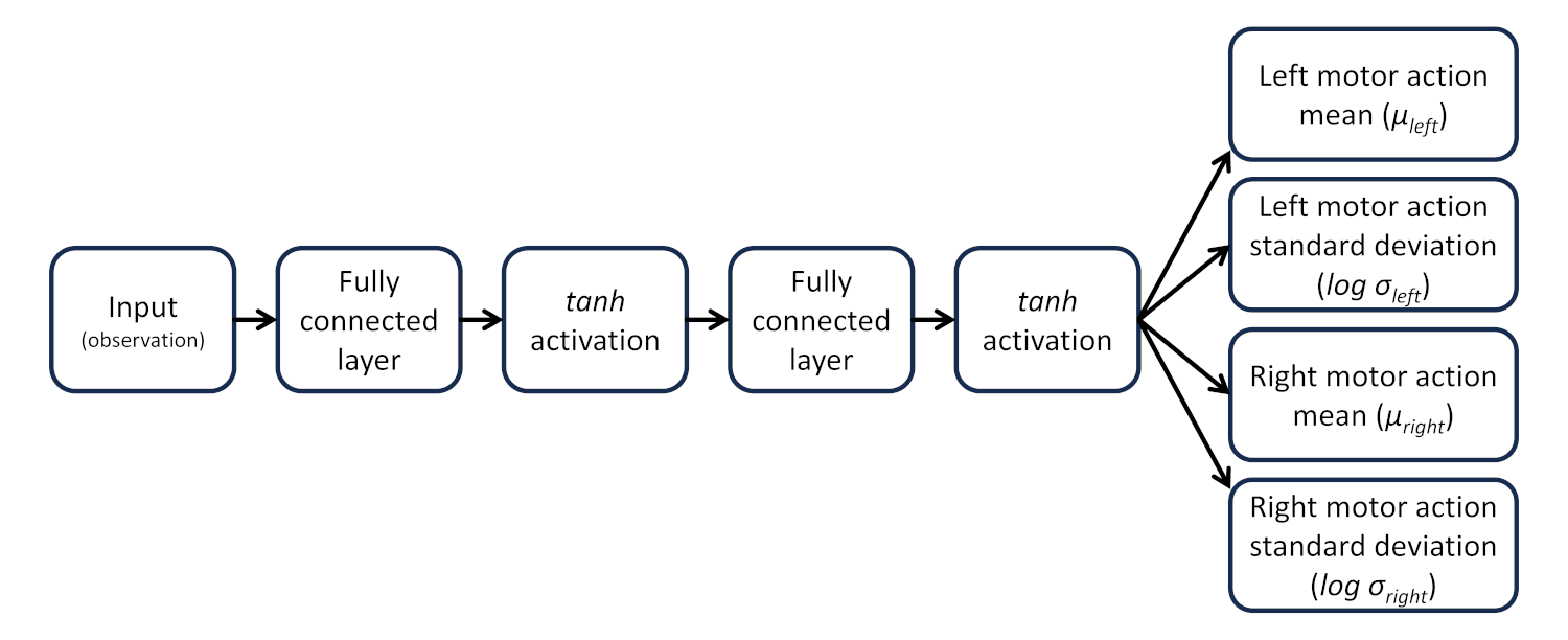
You can then convert the normalized [-1, 1] output to motor control by sampling from the distribution and multiplying by the e.g. pulse width modulation (PWM) max level. If the motor controller accepts -255 to 255 as input (for full reverse speed to full forward speed), you first sample from the distribution and then multiply the output by 255 and clip it to -255 to 255. If we look at just the left motor:
actionleft ~ N(μleft, σleft)
clippedleft = clip(255 ⋅ actionleft, -255, 255)
You would repeat the process for the right motor to get the balance bot control.
In addition to allowing for continuous action spaces, outputting a distribution for each action has the advantage of built-in exploration. No more bolting a random ε chance to take a different action onto the policy. A large standard deviation (σ) encourages a large possibility of exploration around the mean (μ). As the policy learns over time, the distribution can eventually collapse to the mean (i.e. σ = 0), which means the policy has converged to a deterministic policy: always choose the action μ given a particular input state (observation) s.
Why Gaussian rather than, say, a uniform distribution? While other distributions might work, a Gaussian distribution is continuous with a definite peak (the mean). This provides a strong training signal when computing the gradient (as we’ll see later). The gradient of the policy is proportional to how far the sampled action is from the mean, which gives a clear direction to adjust the parameters θ in order to move the mean closer to an action (that should produce a better total return).
Expected Return
With the idea that the policy can be approximated by an arbitrary function, how do we go about defining that function? As we already saw, we can use a neural network, which means updating the parameters θ such that the outputs provide the best possible action(s) given an input s.
In supervised learning, this requires having a set of known-good examples that can be compared to the predicted output. We try to minimize the loss function, a measure of the difference between the predicted output and the known-good samples. In DQN, we defined the loss as the mean squared error between the TD target (r + γ · maxa Q(s’, a; θ)) and the current predicted Q(s,a) over a minibatch of sampled steps.
When it comes to approximating the policy, we do not have the luxury of known-good values to compare actions to. As a result, we need to think differently about what we’re optimizing. Instead of minimizing a loss function, what if we maximized the expected return? That means instead of performing gradient descent (as you normally do when training NNs in supervised learning), we need to perform gradient ascent.
Let’s define J(θ) to be the expected return under policy π, given a set of parameters θ.
\(J(\boldsymbol{\theta}) = \sum_{\tau} p(\tau; \boldsymbol{\theta}) \cdot G(\tau) = \mathbb{E}_{s_0 \sim p(s_0)} \left[ v_{\pi_{\boldsymbol{\theta}}}(s_0) \right]\)
To calculate the expected return of a policy, J(θ), we can sum over all trajectories (τ), weighted by the return of each trajectory (G(τ)). This summation can be found in the middle of the equation. This looks similar to the expected return equation we established in part 4. However, Eπ[Gt] gives the expected return at a given timestep t. In contrast, we want J(θ) to give us the expected return for the entire trajectory, starting at some state st=0.
Note that G(τ) is just G0: the discounted return starting from the very beginning of the episode. We write it as G(τ) here to show that we’re reasoning about whole trajectories as single objects.
The right side of the equation demonstrates another way to think about what J(θ) means: we can rewrite the same definition as the expected return from all possible starting states. In other words, we simply sum the probabilities of starting in some state s0, weighted by the state value of that state (v(s0)).
Writing s0 ~ p(s0) explicitly shows that the starting state is random, but not something the policy has any influence over. It is determined entirely by the environment, before the agent has taken a single action. As we’ll see in the derivation ahead, p(s0) drops out when we differentiate with respect to θ.
For gradient ascent to work, we need to calculate the gradient of the expected return of the policy (with respect to θ): ∇θJ(θ). The problem is that differentiating Στ p(τ; θ) · G(τ) is tricky, as the θ term is inside the probability distribution p(τ; θ). We can use some math tricks to help perform this operation, where a simple numerical differentiation might be normally impossible.
Policy Gradient Theorem
Let’s walk through the derivation of the policy gradient. I found that taking the time to complete this proof was very helpful to wrap my head around what the policy gradient is trying to accomplish.
As a reminder, we are trying to maximize the expected return from any given starting state (s0) by adjusting the parameters (θ) in a policy approximation function (πθ(a|s)). We can do that via gradient ascent, which requires us to compute the gradient of the expected return (∇θJ(θ)).
In the previous post, we used the Q(s,a;θ) notation to follow DQN’s convention. We’ll continue to use that notation for the policy, π(a|s;θ), but note that you’ll often see this written as πθ(a|s) in other RL literature. They mean the same thing.
It is impossible to differentiate J(θ) using the form we presented in the previous section, as the θ term is inside a probability distribution. The goal of this derivation is to manipulate the definition of J(θ) to get it into a form that we can differentiate to solve for the gradient.
We start with the definition of the expected return under policy π and use the sum rule from calculus to move the gradient term inside the summation. G(τ) is not dependent on θ, so we can treat it like a constant, allowing this to work.
\( \nabla_{\boldsymbol{\theta}} J(\boldsymbol{\theta}) = \nabla_{\boldsymbol{\theta}} \sum_{\tau} p(\tau; \boldsymbol{\theta}) \, G(\tau) = \sum_{\tau} \nabla_{\boldsymbol{\theta}} p(\tau; \boldsymbol{\theta}) \cdot G(\tau) \)
We then use the chain rule for logarithms from calculus to define the gradient of log p(τ; θ).
\(\nabla_{\boldsymbol{\theta}} \left[ \log p(\tau; \boldsymbol{\theta}) \right] = \frac{\nabla_{\boldsymbol{\theta}} p(\tau; \boldsymbol{\theta})}{p(\tau; \boldsymbol{\theta})}\)
Note that this requires p(τ; θ) > 0, which works, as we only consider trajectories with a nonzero chance of occurring.
We can rearrange this equation to get a definition for ∇θ p(τ; θ):
\(\nabla_{\boldsymbol{\theta}} p(\tau; \boldsymbol{\theta}) = p(\tau; \boldsymbol{\theta}) \cdot \nabla_{\boldsymbol{\theta}} \log p(\tau; \boldsymbol{\theta})\)
We then substitute this definition in for ∇θ p(τ; θ) in our definition of ∇θJ(θ):
\(\nabla_{\boldsymbol{\theta}} J(\boldsymbol{\theta}) = \sum_{\tau} p(\tau; \boldsymbol{\theta}) \cdot \nabla_{\boldsymbol{\theta}} \log p(\tau; \boldsymbol{\theta}) \cdot G(\tau)\)
What was the reason for this substitution? If you look at the shape of the equation, we now have: Στ p(τ; θ) · [something]. If you recall from part 4, this looks exactly like the definition for expected value: summing over all probabilities, weighted by the value. We can rewrite this using the expected value notation:
\(\nabla J(\boldsymbol{\theta}) = \mathbb{E}_{\tau \sim \pi_{\boldsymbol{\theta}}} \left[ \nabla_{\boldsymbol{\theta}} \log p(\tau; \boldsymbol{\theta}) \cdot G(\tau) \right]\)
The τ~πθ notation shows that τ is a random variable, sampled according to πθ. This is shorthand for saying τ is distributed according to p(τ;θ), the full trajectory probability from post 3. In other words, τ is the trajectory you’d get by actually running the current policy πθ in the environment.
As we discussed in the post on Monte Carlo methods, the law of large numbers states that we can sample from experience enough times that we eventually converge on the expected value. By rewriting ∇θJ(θ) as an expected value, we can now estimate the gradient via sampling rather than having to calculate it analytically.
So, what do we sample? Just like we’ve been doing for the past few algorithms we covered, we use the current policy (πθ) to generate data, where we record a replay buffer containing information about each timestep (S, A, R, S’). We then use that information to compute ∇θ log p(τ;θ) · G(τ) for each episode. We then average this value across several episodes to get an estimate for ∇θJ(θ).
This begs the next question: while we can sum the rewards for the episode to get G(τ), how do we calculate ∇θ log p(τ;θ)? We need to use more math trickery to get this into a form we can actually use.
From post 3, we showed that the probability of a particular trajectory is defined as follows:
\(p(\tau; \boldsymbol{\theta}) = p(s_0) \cdot \prod_{t} \pi(a_t | s_t; \boldsymbol{\theta}) \cdot p(s_{t+1} | s_t, a_t)\)
The product rule of logarithms states that the log of a product is equal to the sum of logs. Therefore, we can rewrite the previous equation as follows:
\(\log p(\tau; \boldsymbol{\theta}) = \log p(s_0) + \sum_{t} \log \pi(a_t | s_t; \boldsymbol{\theta}) + \sum_{t} \log p(s_{t+1} | s_t, a_t)\)
We then find the gradient ∇θ log p(τ;θ) by applying the gradient to all three terms on the right side of the equation.
\(\nabla_{\boldsymbol{\theta}} \log p(\tau; \boldsymbol{\theta}) = \nabla_{\boldsymbol{\theta}} \log p(s_0) + \sum_{t} \nabla_{\boldsymbol{\theta}} \log \pi(a_t | s_t; \boldsymbol{\theta}) + \sum_{t} \nabla_{\boldsymbol{\theta}} \log p(s_{t+1} | s_t, a_t) \)
θ is the variable of differentiation in this context, so any term that does not rely on θ as a variable is considered a constant (for the purpose of differentiation). And from calculus, we know that the derivative of a constant is 0. As a result, two of the terms are actually 0:
- p(s0) – the environment’s initial state distribution, which has nothing to do with θ. The environment decides on the starting state, requiring no input from the policy.
- p(st+1|st, at) – the environment’s transition dynamics (i.e. probability of moving to s’ after taking action a from state s). Again, this is determined by the environment and not the policy, which means it does not depend on θ.
By setting those two terms to 0 in the above equation, we end up with the following:
\(\nabla_{\boldsymbol{\theta}} \log p(\tau; \boldsymbol{\theta}) = \sum_{t} \nabla_{\boldsymbol{\theta}} \log \pi(a_t | s_t; \boldsymbol{\theta})\)
π(at|st; θ) is something we have access to: it’s just the policy approximator function! If we’re using a neural network, we can run a forward pass using our recorded states and actions to compute the value. We then take the log of that value to get log π(at|st; θ), and we can use numerical autograd methods (like those found in PyTorch) to compute ∇θ log π(at|st; θ).
To finish out the derivation, we substitute ∇θ log p(τ;θ) = Σt ∇θ log π(at|st; θ) into our expected value formula to get:
\(\nabla J(\boldsymbol{\theta}) = \mathbb{E}_{\tau \sim \pi_{\boldsymbol{\theta}}} \left[ \left( \sum_{t} \nabla_{\boldsymbol{\theta}} \log \pi(a_t | s_t; \boldsymbol{\theta}) \right) \cdot G(\tau) \right]\)
This gives us an equation that we can work with. We’ll need to sample a lot of data to estimate the expected value, but it’s now tractable and model-free, as we no longer need to know the transition dynamics.
The gradient ∇θ log π(at|st; θ) points in the direction that increases the log-probability of the action actually taken. The return G(τ) then scales that direction: a large positive return pushes the update strongly toward that action, and a small positive return gives a weak update. A negative return pushes the update away from it, decreasing its probability instead.
Policy Gradient in Practice
To estimate the policy gradient, we need to perform a few steps.
- We run the policy in the real (or simulated) environment to get a full episode, recording (st, at, rt) in a replay buffer at every step.
- At each timestep, we know (st, at) (it’s what actually happened), and we use them to calculate π(at|st; θ), which is just a forward pass through the neural network. We take the log of that value to get log π(at|st; θ).
- We use an autograd method to numerically estimate the value of ∇θ log π(at|st; θ) at each timestep. This is the same method used by most machine learning libraries (e.g. PyTorch) to compute the gradient during backpropagation.
- Multiply the estimated ∇θ log π(at|st; θ) by the discounted return for the entire episode G(τ).
- Sum these values over the whole trajectory (t=0, 1, …, T-1) to get a single episode’s estimate of ∇θ J(θ).
This is a single episode estimate, which can be random and noisy. To get a better estimate, you would perform several rollouts with the current policy and average the ∇θ J(θ) calculations together:
\(\nabla J(\boldsymbol{\theta}) \approx \frac{1}{N} \sum_{i=1}^{N} \left[ \left( \sum_{t} \nabla_{\boldsymbol{\theta}} \log \pi(a_t^{(i)} | s_t^{(i)}; \boldsymbol{\theta}) \right) \cdot G(\tau^{(i)}) \right]\)
We now have a Monte Carlo estimate of the policy gradient that we can use to update our policy via gradient ascent. In the next post, we’ll see this policy gradient estimation used in practice as part of the REINFORCE algorithm.
Notice that in step 4, we multiply ∇θ log π(at|st; θ) by the same value G(τ) at each timestep (for a given episode). While this works, we can reduce variance (and be more sample efficient) by using the discounted return Gt, looking forward from that timestep t instead. In the next post, we’ll see how this works using something known as the causality trick.
Conclusion
Going from “a policy gradient exists mathematically” to “we can estimate the policy gradient using model-free sampling methods” is a major leap in the world of RL. As you just saw, it required a lot of complex math to get there. The ability to estimate the policy gradient from experience unlocked the next level of deep RL, as we can now use it to optimize a policy directly. It is foundational to modern deep RL algorithms, including REINFORCE and PPO.
If you have any questions or comments, please let me know!